Advertising is a huge industry, with billions spent every year on marketing products. Are these enormous expenditures worth it? The benefits of increased sales and revenues must be at least as large as the increased costs to make it a good investment. In this section, the profit-maximizing level of advertising will be identified and evaluated.
One important point about advertising is the costs associated with advertising expenditures. If advertising works, it increases sales of the product. There are two major costs, the direct costs of advertising and the additional costs associated with increasing production if the advertising is effective. A typical analysis sets the marginal revenues of advertising equal to the marginal costs of advertising
\[MR_A = MC_A.\]
This would be correct if the level of output remained constant. However, the output level will increase if advertising works, and the additional costs of increased output must be taken into account for a comprehensive and correct analysis, as will be shown below.
Graphical Analysis of Advertising
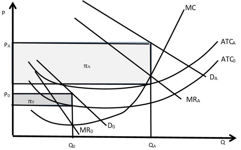
The graph for advertising is shown in Figure \(\PageIndex{1}\). Notice the two major effects of advertising and marketing efforts:
an increase in demand, in this case from \(D_0\) to \(D_A\), and
an increase in costs, shown here as the movement from \(ATC_0\) to \(ATC_A\).
In the analysis shown here, advertising costs are considered to be fixed costs that do not vary with the level of output. This is true for a billboard, or television commercial. Note that the marginal costs do not change, since marginal costs are variable costs. The analysis could be easily extended to include variable advertising costs.
Economic analysis of advertising and marketing is straightforward: continue to advertise as long as the benefits outweigh the costs. In Figure \(\PageIndex{1}\), the optimal level of advertising occurs at quantity \(Q_A\) and price \(P_A\). Profits with advertising are shown by the rectangle \(π_A\). If profits with advertising are larger than profits without advertising \((π_A > π_0)\), then advertising should be undertaken.
Figure \(\PageIndex{1}\): Economic analysis of advertising and marketing.
In general, if the increase in sales \((D_A – D_0)\) is larger than the increase in costs, advertising should be undertaken. The optimal level of advertising can be found using marginal economic analysis, as described in the next section.
General Rule for Advertising
The profit-maximizing level of advertising can be derived, and the outcome is interesting and important, since it diverges from setting the marginal costs of advertising equal to the marginal revenues of advertising. Note that the graphical and mathematical analyses of advertising presented here could be used for any marketing program, not only advertising campaigns.
Assume that the demand for a product is given in Equation \ref{4.4}, where quantity demanded \((Q^d)\) is a function of price \((P)\) and the level of advertising \((A)\).
\[Q^d = Q(P, A) \label{4.4}\]
This demand equation differs from the usual approach of using an inverse demand equation. For this model, it is more useful to use the actual demand equation instead of an inverse demand equation \([P=P(Q^d)]\). The profit equation is shown in Equation \ref{4.5}, where the cost function is given by \(C(Q)\).
\[\begin{align} \max π &= TR – TC \label{4.5}\\[4pt] \max π &= PQ(P, A) – C(Q) – A \end{align}\]
The profit-maximizing level of advertising \((A^*)\) is found by taking the first derivative of the profit function, and setting it equal to zero. This derivative is slightly more complex than usual, since the quantity that appears in the cost function depends on advertising, as shown in Equation \ref{4.4}. Therefore, to find the first derivative, we will need to use the chain rule from calculus, which is used to differentiate a composition of functions, such as the derivative of the function \(f(g(x))\) shown in Equation \ref{4.6}.
The chain rule simply says that to differentiate a composition of functions, first differentiate the outer layer, leaving the inner layer unchanged [the term \(f'(g(x))\)], then differentiate the inner layer [the term \(g'(x)\)].
In Equation \ref{4.5}, the cost function is a composition of the cost function and the demand function: \(C(Q(P, A))\). So the derivative
The term on the left hand side is marginal revenues of advertising \((MR_A)\), and the term on the right hand side is the marginal cost of advertising \((MC_A = 1)\), plus the additional costs associated with producing a larger output to meet the increased demand resulting from advertising [\(MC\cdot\left(\dfrac{∂Q}{∂A}\right)\)].
This result can be used to find an optimal “rule of thumb” for advertising, or a “General Rule for Advertising.” There are three preliminary definitions that will be useful in deriving this important result. First, the advertising to sales ratio is given by \(\dfrac{A}{PQ}\), and reflects the percentage of advertising in total revenues (price multiplied by quantity, \(PQ\)). Second, the advertising elasticity of demand is defined.
Advertising Elasticity of Demand (EA) = The percentage change in quantity demanded resulting from a one percent change in advertising expenditure.
Third, recall the Lerner Index \((L)\), a measure of monopoly power. We derived the relationship between the Lerner Index and the price elasticity of demand, shown in Equation \ref{4.9}:
With these three preliminary equations, we can derive a relatively simple and very useful general rule of advertising from the profit-maximizing condition for advertising, given in Equation \ref{4.7}.
This simple rule states that the profit-maximizing advertising to sales ratio (A/PQ) is equal to minus the elasticity of advertising \((E^A)\) divided by the price elasticity of demand \((–E^d)\). The result is simple and powerful: (1) if the elasticity of advertising is large, increase the advertising to sales ratio, and (2) if the price elasticity of demand is large, decrease the advertising to sale ratio. A firm with monopoly power, or a higher Lerner Index, will want to advertise more (\(E^d\) small), since the marginal profit from each additional dollar of advertising or marketing expenditure is greater.
Most business firms have at least crude approximations of the two elasticities needed to use this simple rule. Many firms advertise less than the optimal rate, since marketing can appear to be expensive if it is a large percentage of sales. However, simple economic principles can be used to determine the optimal, profit-maximizing level of advertising and/or marketing expenditures using this simple rule.