5.2: Intertemporal Consumer Choice

Suppose the government wants to stimulate saving by workers so they won’t be poor when they retire. Individual Retirement Accounts (IRAs) and 401(k) (their section in the tax code) plans enable savings to grow tax free, so the interest rate earned is higher than if returns were taxed. A higher interest rate should stimulate more saving. But how much more?

Typically, estimates of the interest rate elasticity of savings are positive, but quite small, say 0.15. If someone had this elasticity, would attempts to stimulate saving by increasing the interest rate be effective?

No, because the low interest rate elasticity of savings means that saving is not responsive to changes in the interest rate. Suppose the interest rate doubles so we have a huge 100% change. Because the elasticity is 0.15, that means we will see only a 15% increase in savings. A more realistic 10% increase in the interest rate would generate a small 1.5% increase in savings. The small elasticity tells us that shocks to the interest rate are not going to move the amount saved by very much.

This is an example of interpreting an elasticity. Computing an elasticity is important (and you will continue to see examples of how to do it), but understanding what an elasticity is telling us is even more critical.

Now that we know the elasticity is low and what that means, this leads to a second question: What would make the interest rate elasticity of savings be so small? The rest of this chapter offers an application of the Endowment Model to answer this question. In addition, income and substitution effects play a major role in the explanation. There is no doubt about it, learning economics is a cumulative undertakingthe same ideas keep popping up again and again.

The Intertemporal Choice Model

Intertemporal choice means the agent faces a decision that spans across time periods. Saving over the years working means less consumption, but that allows for more consumption when retired. We model the agent as deciding what to consume every year over their lifespan.

Just as when we modeled the consumer buying just \(x_1\) and \(x_2\) instead of many goods and services, we make a simplifying assumption that collapses many time periods into two: present and future. In the present, right now, the agent works and in the future, one year later, she does not (she retires).

In addition, there is another implied simplifying assumption: the agent knows with certainty how long she will live. She is born and works as one-year old, is retired as a two-year old and dies on the last day of her second year. She decides, as soon as she is born, how much she will consume in year 1 (the present) and year 2 (the future).

Instead of having two goods \(x_1\) and \(x_2\), we have consumption of a single good in the present, \(c_1\), and the future, \(c_2\). The price of the single good is $1/unit so if you have, say, $40, you can buy 40 units. There is no inflation so the price is the same in both time periods.

Notice the usual modeling technique at work hererealistic details are simply assumed away. Most people’s lives unfold as follows: Childhood becomes teen-aged years, and then a long period of working adult life eventually turns to retirement years and death. The Intertemporal Choice Model collapses all of that into two time periods. It also assumes away complications from not knowing exactly when we die.

Faced with criticisms about the unrealistic nature of the model, economists respond by saying that we are not interested in realism. We reduce the complex real world to a model that can be analyzed with comparative statics to produce testable predictions. For economists, the goal is not to describe reality, but to predict via comparative statics. We strip away all complications to create an unreal, incredibly simple model that contains the kernel of the problem so we can work out how the agent responds to shocks.

Modeling is not easy. There is science (and math) and art involved. Users and consumers of these models need sharp critical thinking skillssometimes important elements are assumed away.

We continue building the model by defining the initial endowment as the amount of present and future income you start with. The initial endowment in the first year is \(m_1\) and in the second year \(m_2\). The first year’s initial endowment is income from working and the second year’s initial endowment is income from sources like Social Security. Thus, it makes sense that \(m_1 > m_2\), which says that income is higher during the working than the retired year. Since the price is $1/unit, the initial endowment incomes are also initial endowment consumption in the two periods.

We are ready to work on the optimization problem itself. We follow the usual approach, modeling the budget constraint, then satisfaction, then putting the two together to find the initial solution. Of course, after finding the initial optimum we will do comparative statics analysis, where we will answer the question: What causes the interest rate elasticity of savings to be so small?

The Budget Constraint

STEP Open the Excel workbook IntertemporalChoice.xls and read the Intro sheet, then go to the MovingAround sheet.

The consumer begins at the initial endowment point, 80,20, where 80 represents her income and consumption in time period 1 (remember that the price of the good is $1/unit). Income and consumption of 20 in time period 2 is lower (given that she is not working). These numbers are arbitrary and do not have any special meaning.

A critical concept for the Endowment Model is that the agent does not have to stay at the initial position. In this application, she can move by saving or borrowing. Saving means you consume less in the present and carry over the unconsumed portion into the future. Saving is like selling present consumption and buying future consumption.

Suppose she saves 30 units of consumption in year 1 by saving $30. What would be her position in the second year?

STEP Change cell B19 to 50. This implements the plan to increase future consumption, but look at cells B21 and B22. Instead of simply reallocating from 80,20 to 50,50, by saving 30 units, she got an extra 6 units in interest on her savings.

If you save $30 for one year at 20%, you end up with $56. The $30 you saved (called the principal) and interest earned of $30 x 20% = $6 makes your savings worth $36 in the future and we add this to the $20 of initial future income to get the grand total of $56.

There is an equation that gives us the value of \(c_2\) for any chosen value of \(c_1\). \[c_2 = m_2 + (m_1 - c_1) + r(m_1 - c_1)\] The equation says that the amount of consumption in time period 2 equals the initial endowment amount in time period 2, \(m_2\), plus the principal saved, \(m_1 - c_1\), plus the interest earned on the amount saved, \(r(m_1 - c_1)\). We can rewrite this in a simpler form by collecting the savings term. \[c_2 = m_2 + (1+ r)(m_1 - c_1)\] This is the equation of the budget constraint in this model. It shows that the intercept is \(m_2 + (1+ r)m_1\) and the slope is \(-(1+r)\) (just multiply through by \((1+r)\)). The slope tells us that saving $1 will yield \(1 + r\) dollars in time period 2.

What would be the maximum consumption possible in time period 2? We have two ways to answer this question.

STEP Change cell B19 to 0. She consumes nothing now and ends up with 116 units in the future.

"But she will starve if she consumes nothing in period 1." That would be another constraint that is not being modeled. We are not saying she will consume nothing in the present time period, we are merely exploring the consumption possibilities.

Saving everything (the same as consuming nothing in the present) can also be found by computing the value of the y intercept. We can evaluate \(m_2 + (1+ r)m_1\) at \(m_1 = 80, m_2 = 20\), and \(r=20\%\), yielding \(20 + (1+0.2)80 = 116\). This is the same answer that we got with Excel.

The y intercept tells us the future value of the agent’s initial endowment, measuring income in both periods in terms of time period 2.

Instead of saving, the agent can borrow. Suppose the agent decided to consume more than 80 units in time period 1. How could she do this? Easy: use her time period 2 income to borrow from it. As before, however, we have to be careful. The interest rate plays a role.

STEP Change cell B19 to 90. She borrows $10 from her future income.

Does she end up with 90,10subtracting 10 from \(c_2\) and adding it to \(c_1\)? No way. As Excel shows, she has to pay interest on the borrowed funds. If she borrows $10, she ends up with only $8 in the future because she has to pay back the principal ($10) and the interest ($2).

What is the most she could consume in time period 1?

STEP Change cell B19 to 100. What happens?

She cannot do this. She cannot choose negative \(x_2\). She does not have enough future income to enable 100 units of time period 1 consumption.

STEP Continue entering numbers in cell B19 until you drive \(c_2\) (in cells B23 and B24) to zero.

The x intercept is \(96 \frac{2}{3}\). It is the present value of her endowment, measuring income in both periods from the standpoint of time period 1.

STEP Proceed to the Properties sheet.

Our work in the MovingAround sheet makes it easy to understand the budget line displayed in the Properties sheet. Clearly, given an initial endowment, movement up the budget line is saving and down is borrowing.

These are just consumption possibilities. We do not know what this person will do until we incorporate her preferences. We do know she can be anywhere on the constraint (including the initial endowment point). It all depends on her indifference map and where the highest attainable indifference curves lie.

STEP Proceed to the Changes sheet. Change the interest rate, cell L8, to 50%. Your screen will look like Figure 5.5.

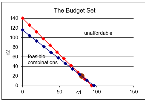
Figure 5.5: Increasing r. Source: IntertemporalChoice.xls!Changes

Our work with the Endowment Model in the previous section enables us to easily interpret the result. As before, the budget constraint swivels around the initial endowment point.

Above the initial endowment point, the increase in r is a good thing, increasing consumption possibilities. If the agent is a saver, the shock is welcome.

Borrowers, however, would not be happy with an increase in r. This is a price increase to present consumption and reduces consumption possibilities for borrowers.

STEP Click the button. Change \(m_1\) and \(m_2\) to see how these shocks are like an income shock. It maintains the slope, but shifts the budget constraint.

Now that we understand how the budget constraint works, we are ready to turn to the agent’s goal, maximizing utility.

Preferences

The agent has preferences over present and future consumption that can be captured by the indifference map.

We use the usual Cobb-Douglas function form to express preferences as a utility function.

STEP Proceed to the Preferences sheet. Compare the utility functions with d = 0.5 and d = 0.1. The utility function allows us to model different preferences.

Figure 5.6 shows two different agents with different rates of time preference for future consumption. The person on the right exhibits a strong preference for present consumption, while the person on the left is more willing to wait.

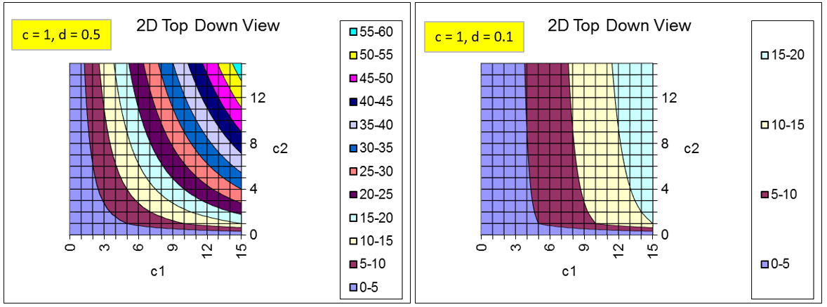
Figure 5.6: Modeling rates of time preference. Source: IntertemporalChoice.xls!Preferences

A more immediate gratification personality is represented on the right side of Figure 5.6. We would say this person is more impatienthe likes present much more than future consumption. The exponent d is much smaller than c, which means inputs into the utility function through \(c_2\) provide much less utility than via \(c_1\).

The steep indifference curves reveal that he is willing to trade a great deal of future consumption for a just a little more present consumption. His MRS at a given point (for example, 6,6) is higher (in absolute value) than the MRS of the person on the left.

We do not say the person on the right has "bad preferences" (although the language used in this example, such as impatience does seem to connote disapproval). Economists take preferences as given. We are not supposed to judge them as right or wrong. A person with preferences that substantially ignore the future is treated the same as someone who does not like broccoli or likes the color blue.

There is a complication here, however, in that a person’s rate of time preference almost certainly changes over time. A young person may not save much because she does not value the future, but she may regret her decision when she gets older. Deciding whose preferences should rule, young or old you, is a difficult philosophical problem.

With the budget line and preferences, we can now solve the constrained utility maximization problem.

Finding the Initial Solution

STEP Proceed to the OptimalChoice sheet. Figure 5.7 shows the initial display. The current bundle is 80,20the initial endowment point. The agent is not maximizing satisfaction subject to the budget constraint. The indifference curve is clearly cutting the budget line and, therefore, the agent should move northwest up the budget line to maximize utility.

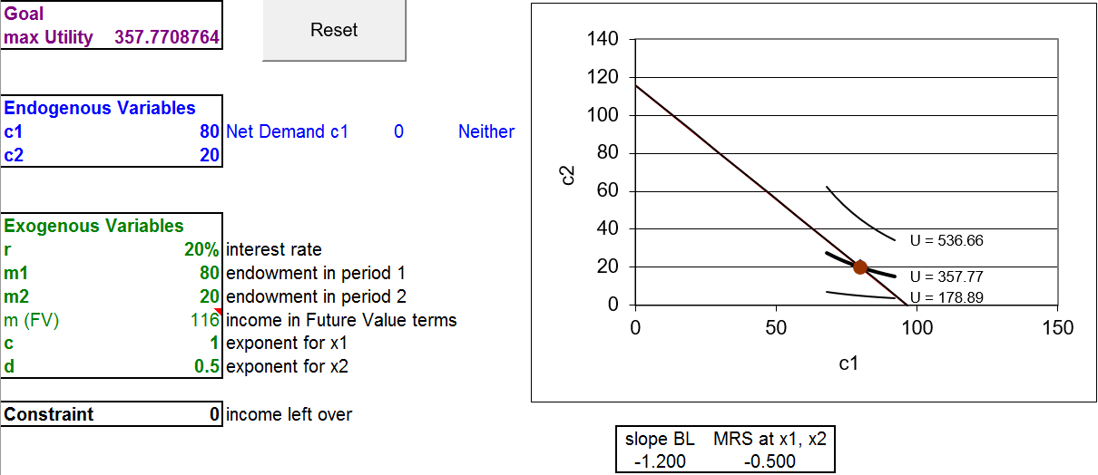
Figure 5.7: An inefficient position. Source: IntertemporalChoice.xls!OptimalChoice

Run Solver to find the initial solution.

The agent opts for the point \(64 \frac{4}{9},38 \frac{2}{3}\). This means she has decided to save \(15 \frac{5}{9}\) of her present consumption. She chooses this present and future combination, implying this level of saving, because this maximizes utility subject to the budget constraint.

Notice that the negative net demand is interpreted as saving. It is computed as optimal \(c_1\) minus the initial endowment of present consumption. As mentioned earlier, saving is like selling present consumption to buy greater future consumption. We often drop the minus sign so we do not get confused by increases and decreases in saving.

Comparative Statics

We focus on \(r\). We want to know how savings will respond when \(r\) changes. Remember our question: Why is the interest rate elasticity of savings so low?

Before we begin our comparative statics analysis, we need to be clear about the language used. Since the shock variable, \(r\), is measured as a percent, things can get confusing once we start working on responses and elasticities. We need to keep clear the difference between a percentage point change and percent change. They sound the same, but the former is a difference (\(\Delta\)), \(\text{new} - \text{inital}\), and the latter is a percent computation,

\[\dfrac{\text{new} - \text{initial}}{\text{initial}}. \nonumber\]

So, if \(r\) increases from 20% to 30%, that is a 10 percentage point change since we compute 30 - 20, but a 50 percent change: \(\frac{30-20}{20}\). The same language would be used if we were working with unemployment rates. An increase from 5% to 6% is a one percentage point increase and a 20% increase.

The finance literature uses basis points for differences in variables measured in percents. There are 100 basis points in one percentage point. If a bond yield rises from 3.25% to 3.35%, that is an increase of 10 basis points.

STEP Run the Comparative Statics Wizard, changing the interest rate by 10 percentage points (0.1) increments. Keep track of \(c_1\), \(c_2\), net demand, and whether the person is a saver or borrower (cells D11 and E11).

Your results should be similar to those in the CSr sheet.

STEP Use your CSWiz results to compute the interest rate elasticity of savings from r = 20% to 30%.

We find that the interest rate elasticity of savings from r = 20% to 30% is about 0.11. (Check the formula in cell I15 in the CSr sheet if needed.) That is quite low. A 50 percent increase in r only increased savings by a little over 5 percent.

This elasticity is similar to the 0.15 elasticity at the beginning of this chapter. Why is this happening? Why is saving so unresponsive to changes in the interest rate?

The answer lies in the income and substitution effects. For savings, the income and substitution effects from a change in r work in opposite directions (when \(c_1\) is a normal good). Thus, they tend to cancel each other out and the total effect ends up being small.

To head off serious misunderstanding, you need to know right now that this does not mean that we are dealing with a Giffen good. We will see that we are dealing with cross effects when r rises for a saver and Giffen goods are defined in terms of own effects. Also, \(c_1\) and \(c_2\) are both normal goods in a Cobb-Douglas utility function so we know we can’t get Giffenness.

STEP To see how the income and substitution effects apply to this problem, return to the OptimalChoice sheet. Suppose r increases to 300%. Change B16 to this absurdly high interest rate.

This huge change enables us to see clearly what is happening on the graph. The budget line swivels in a clockwise direction, getting much steeper. Remember that the slope is \(-(1+r)\) so an increase in r makes the line steeper. This is good for savers and bad for borrowers.

STEP After changing cell B16 to 300%, run Solver to find the new initial solution.

Solver gives the new optimal solution, \(c_1 \mbox{*} = 56 \frac{2}{3}\) and \(c_2 \mbox{*}=113 \frac{1}{3}\), when \(r=300\%\). Optimal savings has increased from $15.56 to $23.33, so that is good news, but this is a pretty weak response to the massive increase in the interest rate from 20% to 300%.

Figure 5.8 shows the initial solution (point A) and the new optimal solution (point C). It also includes a dashed line that is parallel to point C’s budget line, but goes through point A. This, of course, is the line that is used to separate the total effect into income and substitution effects using point B.

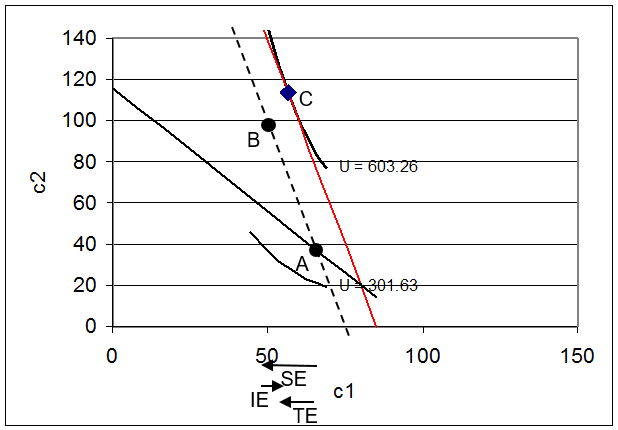
Figure 5.8: Income and substitution effects. Source: IntertemporalChoice.xls!OptimalChoice: cell F52

How much income (\(m_1\)) did we have to take away (hypothetically, of course) to cancel out the income effect of the higher interest rate? We can use Excel to answer this question.

STEP With r = 300%, enter the initial solution (point A). To minimize rounding error, use a formula with fractions. So, enter "= 64 + 4/9" in B11 and "= 38 + 2/3" in B12. Now, start decreasing \(m_1\) (in cell B17). Your goal is to find that value of \(m_1\) so that the initial solution is on the budget linei.e., the constraint cell is zero.

A little experimentation should convince you that \(m_1 = 69 \frac{1}{9}\) is the value that puts the dashed budget line through the initial solution.

If you want to be daring, you could use Solver. Call Solver, then click the button. The objective is the constraint cell (B23) and you want to make the value of it zero by changing \(m_1\) (B17). Solver gives the same answer as above.

Or, you could use the budget constraint to find the \(m_1\) needed to buy the original optimal bundle with \(r= 300\%\). Simply plug in the initial optimal solution along with the new value of r (and initial \(m_2\)) and solve for \(m_1\). You are finding the value of \(m_1\) that would enable you to buy the initial optimal combination with the higher interest rate. The analytical answer agrees with the numerical approach.

STEP Now, with r = 300% and \(m_1 = 69 \frac{1}{9}\), run Solver to find point B.

Be careful with the interpretation of savings for point B. Remember that income is not really \(m_1 = 69 \frac{1}{9}\), but 80. This means that at point B, the agent would save $30.59, not $19.07 as displayed in cell D11.

Figure 5.9 shows the results in a table. You can see Figures 5.8 and 5.9 side by side by scrolling down to row 50 or so in the OptimalChoice sheet. Look at how the substitution effect leads to a large increase in savings, but the income effect cancels out part of this increase.

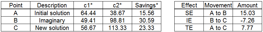
Figure 5.9: Total, income, and substitution effects. Source: IntertemporalChoice.xls!OptimalChoice: cell M51

The income and substitution effects provide an explanation for the low interest rate elasticity of savings. What is happening is that the two effects are working against each other when r rises and the agent is a saver.

Does this mean \(c_1\) is an inferior good? No. The reason why the effects are opposing each other is because, for savers, an increase in the interest rate is like a decrease in the price of future consumption so the effects on \(c_1\) and savings are actually cross effects. Look carefully at Figure 5.8. In the region of the graph with points A, B, and C, it is as if we decreased \(p_2\),and rotated the budget line up clockwise (with a steeper slope).

Saving and Borrowing Explained

The Intertemporal Choice Model is an application of the Endowment Model in the Theory of Consumer Behavior. The model says that the agent chooses the amount to consume in time periods 1 and 2 in order to maximize satisfaction given a budget constraint.

The model explains saving (or borrowing) as an optimizing move on the part of an agent who is trading off present and future consumption.

The model can also explain why the interest rate elasticity of savings is often estimated as a positive, but small number, which means that saving is quite unresponsive to the interest rate. The explanation rests on the fact that the income effect opposes the substitution effect for \(c_1\) and savings (for those with negative net demand for \(c_1\)).

Exercises

1. Solve the problem in the OptimalChoice sheet using analytical methods. In other words, find the reduced form expressions for optimal \(c_1\), \(c_2\), and saving from \[
   \begin{aligned}
   &\max _{c_{1}, c_{2}} u\left(c_{1}, c_{2}\right)=c_{1}^{c} c_{2}^{d} \\
   &\text { s.t. } c_{2}=m_{2}+(1+\mathrm{r})\left(m_{1}-c_{1}\right)
   \end{aligned}
   \]

   Show your work.

2. Use the parameter values in the OptimalChoice sheet (with r = 20%) to evaluate your answers for question 1. Provide numerical answers for the optimal combination of consumption in time periods 1 and 2 and for optimal saving.
3. Do your answers from question 2 agree with Excel’s Solver results? Is this surprising? Explain.
4. Use your reduced form solution from question 1 to compute the interest rate elasticity of savings at r = 20%.
5. In working through this chapter, you found the interest rate elasticity of savings from r = 20% to 30%. Why is the elasticity computed at a point (in question 4 above) different from this elasticity?

References

The epigraph is on page 66 of Irving Fisher, The Theory of Interest: As Determined by Impatience to Spend Income and Opportunity to Invest It (first edition, 1930; reprinted 1977 by Porcupine Press).

Joseph Schumpeter had high praise for Fisher: "[S]ome future historian may well consider Fisher as the greatest of America’s scientific economists up to our own day" (History of Economic Analysis, 1954, p. 872). Schumpeter chose to ignore Fisher’s "propagandist activities (temperance, eugenics, hygiene, and others)," but he did point out that Fisher’s reputation as an economist was negatively affected: "Fisher, a reformer of the highest and purest type, never counted costseven those most intensive pain costs which consist in being looked upon as something of a crankand his fame as a scientist suffered correspondingly" (History of Economic Analysis, 1954, p. 873).

For a recent biography of Fisher, who seems to be enjoying a rehabilitation of sorts, see Robert W. Dimand (2019), Irving Fisher.

The empirical evidence on the interest rate elasticity of savings is mixed (which is actually evidence that it is not large). For a dated, but perhaps comprehensible example, see Irwin Friend and Joel Hasbrouck, “Saving and After-Tax Rates of Return,” The Review of Economics and Statistics, Vol. 65, No. 4. (November, 1983), pp. 537–543, www.jstor.org/stable/1935921.

The literature on the effect of Individual Retirement Accounts and other plans (such as 401(k)) on saving is truly vast. A Google Scholar search on "individual retirement accounts saving" produces hundreds of thousands of hits. This topic would make an excellent paper or undergraduate senior thesis.