11: Inflation, real GDP, monetary policy and fiscal policy
- Page ID
- 45496
Chapter 11: Inflation, real GDP, monetary policy & fiscal policy
In this chapter we will explore:
| 11.1 | Inflation and aggregate demand |
| 11.2 | Aggregate supply |
| 11.3 | The equilibrium inflation rate |
| 11.4 | Adjustment to output gaps |
| 11.5 | Monetary & fiscal policy |
| 11.6 | Recession, disinflation and deflation |
Chapter 4 identified the inflation rate, the unemployment rate and the GDP growth rate as key indicators of economic performance. This chapter combines the concepts of earlier chapters into a full basic macroeconomic model of the economy for the study of causes of change in the first two of these indicators. It is representative of the models currently used by central banks and policy analysts to evaluate current economic performance and policy, forecast future performance and prescribe policy action. Economic growth and growth rates are covered in Chapter 13.
Underlying short-run conditions on the supply side of the economy are the same in this chapter as in earlier chapters. Labour force and technology are fixed by assumption, fixing potential output at YP. Instead of a fixed short-term equilibrium price level, the modern model assumes equilibrium rates of change in money wage rates, and inflation rates are stable in the short run and adjust slowly to output gaps.
On the demand side, monetary policy is aimed at inflation control using the short-term interest rate as the instrument as explained in Chapter 10. It reflects current Bank of Canada monetary policy as explained by the Bank at: www.bankofcanada.ca/core-functions/monetary-policy/. In normal conditions this allows fiscal policy to target the budget deficit and public debt ratio.
The model provides explanations of business cycle fluctuations in output, employment and inflation rates. It also provides a basis for evaluating recent changes in economic conditions and monetary and fiscal policy actions.
11.1 Inflation and aggregate demand
Monetary policy establishes the link between the inflation rate and aggregate expenditure that determines the slope of the AD curve. Central banks set interest rates to control the inflation rate based on an inflation rate target. A monetary policy that reacts to changes in the inflation rate by changing the interest rate causes changes in expenditures. The link between the inflation rate and aggregate expenditure still comes through interest rates and the monetary transmission mechanism, but it is the central bank's decision to change its policy interest rate that provides the impulse.
Changes in autonomous expenditure that are independent of interest rates are still an important part of aggregate demand. They cause shifts in the AD curve based on the multiplier as explained in earlier chapters. Changes in government fiscal policy and in the central bank setting of its interest rate target also shift AD. It is the monetary policy response to transitory variations in the inflation rate that give the AD curve its slope.
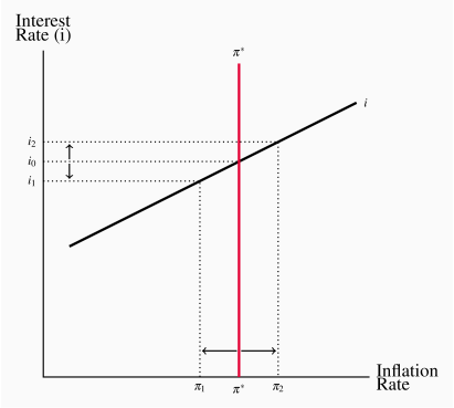
Figure 11.1 illustrates this monetary policy. Assume the central bank has an inflation control target such as  . Based on its evaluation of current and near future aggregate expenditure and supply conditions the Bank sets the interest rate i0 to get its target inflation rate. If the actual inflation rate differs from
  as a result of changes in economic conditions that the Bank views as temporary, rather than fundamental, it reacts with temporary changes in its interest rate within a narrow range, allowing some variation around i0 such as i1 to i2. The Bank of Canada, for example, sets its overnight rate as the midpoint between the bank rate and the deposit rate. The upward sloping line in the diagram shows this 'reaction function'.
 .
.This is a simple policy rule you will recall from Chapter 10. An equation that describes this policy rule would be:
 | (11.1) |
 . An economy working at potential output would have a constant inflation rate
  at i0.
 , the stronger the Bank's reaction to short-term variation in the inflation rate and the steeper the interest rate line.
Alternatively if the Bank does not react to temporary departures from  , that is if
  , the interest rate line is horizontal. Changes in the Bank's official setting of the overnight rate would then shift the interest rate line up or down as the case may be.
This approach to monetary policy and the inflation rate aggregate demand is based on two familiar relationships:
The monetary transmission mechanism as in Chapter 9, and
The expenditure multiplier from Chapters 6 & 7.
Figure 11.2 shows the derivation of the aggregate demand curve labelled AD . This is to differentiate it from the AD curve in Figure 9.5. In that example and examples in earlier chapters in which the equilibrium price level was constant, the inflation rate was zero, and a change in the money supply shifted the AD curve.
 function
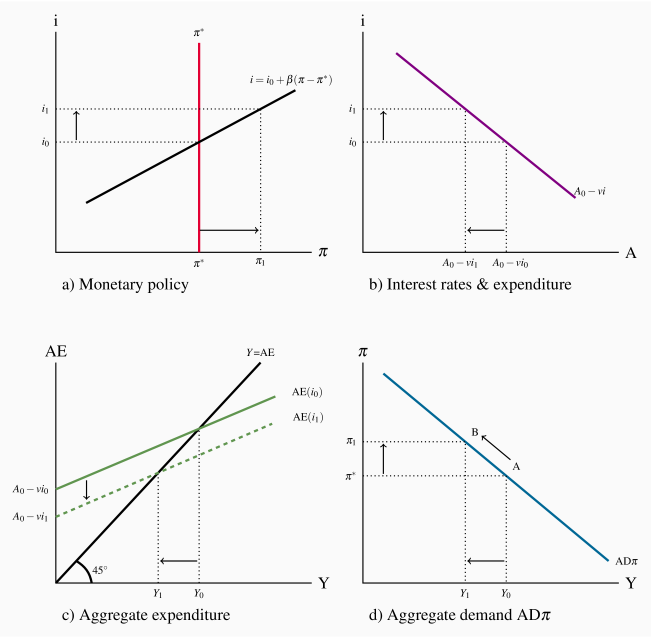
 and interest rate i=i0 in a), and
  and Y0 at A in d). Suppose the inflation rate rises to
  . The central bank then raises its interest rate to i1. The higher interest rate reduces expenditure in b), lowering AE in c) and equilibrium real GDP to Y1. The new equilibrium combination
  is point B on the
  curve.
Figure 11.2 illustrates the relationship between the inflation rate, monetary policy and the slope of the  curve. In this example the central bank does react to temporary variations in
  , (
, ( ). Monetary policy as described by a policy rule or reaction function like Equation 11.1 is in Panel a) of the diagram. Interest rates set by policy in Panel a) determine autonomous expenditures in Panel b) giving the monetary transmission mechanism. Autonomous expenditures determine the position of the AE line in Panel c) and work through the multiplier to determine equilibrium real GDP. The combination of the inflation rate
  and equilibrium real GDP, Y0, give one point
  on an
on an  curve plotted in Panel d) and labeled A.
The central bank's reactions to changes in the inflation rate, other things constant, move the economy along the  function. In Panel a) the Bank reacts to a temporary or transitory rise in the inflation rate to
  by allowing its policy interest rate to rise to i1. This reduces autonomous expenditure in Panel b) to A0–vi1 and lowers the AE curve in Panel c) to
  . The multiplier then lowers equilibrium real GDP to Y1 and plotting
  in Panel d) gives a second point on an
  curve labeled B.
Changes in autonomous expenditures ( ) not caused by changes in interest rates, like changes in autonomous consumption, investment, exports, or government expenditure would shift the
  function by amounts driven by the multiplier. Similarly, a change in monetary policy made by changing i0, in response to a change in economic fundamentals would shift the
  function.
The recession of 2009, for example, brought a sharp drop in Canadian exports and a shift in  to the left. The Bank of Canada lowered its setting for the overnight interest rate in steps from 4.75 percent to 0.25 percent, as illustrated in Figure 10.2, to offset some of this drop in
  . However the monetary stimulus to
  through lower interest rates was not enough by itself to avoid a recession. Fiscal stimulus was also needed.
11.2 Aggregate supply
The supply side of the economy explains output, inflation, and the economy's adjustment to equilibrium at YP, potential output. If the economy is operating with an output gap, changes in the rate of increase in wage rates and other factor prices may push the economy toward a long-run equilibrium at potential output and a constant rate of inflation. But this internal adjustment process is slow at best.
No matter what time frame we use, the economy's output depends on:
The state of technology;
The quantities of factor inputs to production (labour, capital, land, energy, and entrepreneurship); and
The efficiency with which resources and technology are used.
A simple production function defines the relationship between outputs and labour and capital inputs to production as follows:
 | (11.2) |
In this equation, Y is real GDP, A is the state of technology, and N and K are inputs of labour and capital, respectively, used in the production process.
Production function: outputs determined by technology and inputs of labour and capital.
The notation F(...) tells us that the size of output as measured by real GDP depends on the amount of labour and capital used in the production process. More labour and more capital used means more output. An improvement in technology would make A larger, and increase the output produced by any given amount of labour and capital employed. This would be an increase in productivity, an increase in output per unit of input.
Productivity: output per unit of input.
Long-run aggregate supply (YP)
Potential output (YP) is determined by the current state of technology, A0, the current stock of capital, K0, and the equilibrium level of employment, NF. In terms of the simple production function, this means:

Potential output (YP): the real GDP the economy can produce on a sustained basis with current labour capital and technology without generating inflationary pressure on prices.
The short-run fluctuations in output studied in earlier chapters are linked to differences between actual labour input N and the "full employment" labour input NF. Unemployment rates fluctuate as a result of these changes in actual output and employment relative to potential output.
Short-run aggregate supply
Short-run aggregate supply in the 'modern' model defines the relationship between output and the inflation rate, when capital stock, technology and the rate of growth in money wages are fixed. The basic argument is that monopolistically competitive firms set prices at a mark-up over marginal costs of production. The rates of increase in marginal costs of production depend in turn on the rates of increase in money wage rates, prices of material inputs, and productivity.
Prices are sticky in the very short run. Changing prices is costly and competition among producers means relative prices are important to market position. Furthermore, stable prices may help to build customer loyalty. As a result, price changes only follow changes in costs that last beyond the current short term. A horizontal short-run aggregate supply curve as in Figure 11.3 captures this output-inflation relationship.
Persistently strong aggregate demand would increase employment, output and capacity utilization, and lower productivity. Employment would rise and the unemployment rate would fall below the NAIRU, increasing the growth in money wage rates. This upward pressure on current and future marginal costs would compress producers' markups and profitability. Alternatively, persistently weak aggregate demand would lower rates of increase in money wage rates, lower material costs, lower marginal costs, and increase mark-ups. Producers wouldn't adjust price setting practices immediately in either case. But they would react if their mark-ups are persistently pushed away from what they see as the profit maximizing level.
NAIRU: the 'non-accelerating inflation rate of unemployment' that corresponds to NF at YP.
These short-run aggregate conditions are described in a simple  function that explains the current inflation rate as:
(
 ) The rate of inflation last period or last year.
(
 ) The output gap last period or last year.
(
 ) A term that captures the effects of disturbances such as commodity price shocks or extreme climate conditions or political events that would shift supply conditions.
These factors are combined in an equation along with the parameter  which measures the size of the effect an output gap has on the inflation rate:
 | (11.3) |
Equation 11.3 gives a horizontal short-run  curve that is sometimes called an 'inflation adjustment' function. The current inflation rate (
 ) is 'last year's' inflation rate
  adjusted up or down in reaction to 'last year's' output gap. In other words the inflation rate changes with a lag in response to the effect of an output gap on costs and prices. If there is no output gap, the inflation rate would be the same from year to year. As an alternative,
  could be specified as an upward sloping function by dropping the lag on the output gap, but that would remove some of the short-run stickiness observed in wage rates and prices. Figure 11.3 illustrates potential output (YP) and short-run aggregate supply
  .
.
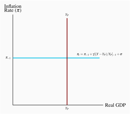
 rate, shifting the line up or down in the next time period.
11.3 The equilibrium inflation rate
Figure 11.4 shows the aggregate demand curve  and the vertical long-run aggregate supply curve YP. Output is at potential output, and the inflation rate,
  , is determined by aggregate demand. At point A there is equilibrium in all markets: for output, money, and labour.
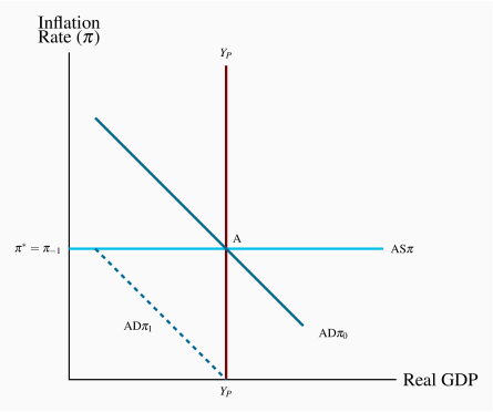
 and YP, as at point A in the diagram. This is also the short-run equilibrium inflation rate. If
  is the central bank's monetary policy target, the bank sets its interest rate to get
  .
. , is determined by autonomous expenditure, fiscal policy, and the monetary policy of the central bank.
 . Then equilibrium is at output YP and the inflation rate
  . This
  curve is not extended below a zero inflation rate. The discussion of deflation, negative inflation rates, on output and policy are important issues covered in Section 11.6.
In practice, central banks do not set zero inflation targets for monetary policy. Some, including the Bank of Canada, set explicit low inflation rate targets. Others, including the United States Federal Reserve, work to implicit inflation rate targets that are also positive and low. There has been and still is a lot of discussion among economists about the appropriate level of the inflation rate target. The Bank of Canada's 2 percent target represents a current consensus on the issue.
The  curve in Figure 11.4 is based on a monetary policy inflation target of
  . In setting its inflation target, the central bank recognizes that money is neutral when wages and prices are flexible and there is no money illusion. This means that the central bank cannot influence potential output, but it can determine the equilibrium inflation rate. It sets the interest rate and accepts growth in the money supply consistent with its inflation target. A rate of inflation,
  , greater than zero means the rate of growth of the money supply,
  , is greater than zero. This puts the
  curve at
  , and keeps it there as inflation raises the price level at the target rate.
11.4 Adjustments to output gaps
Now consider how demand or supply shocks that move the economy away from potential output trigger an adjustment process. In combining the  and
and  curves, it is assumed the market for goods and services clears even in the short run, but the labour market takes longer to adjust. The inflation rate changes over time as wage rate growth adjusts to the unemployment rate. If this process goes smoothly and other conditions are tranquil, it may eventually restore full employment at potential output. But in the meantime output gaps can be quite persistent.
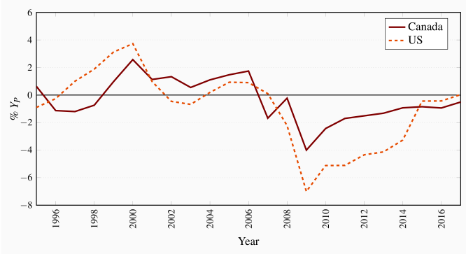
Figure 11.5 provides some empirical evidence. For Canada, the recessionary gap of the last half of the 1990s lasted for about five years. The small inflationary gaps that followed persisted for seven years, and were followed by large recessionary gaps in the financial crisis of 2008–09, which have diminished in size but persist into 2016–17. The data show that automatic adjustments are slow at best.
An aggregate demand shock
Figure 11.6 shows the adjustment to an output gap that is built into the  model. In the diagram, an unexpected fall in aggregate demand shifts the
  function to the left. A decline in exports or investment or government expenditure, or a change in the inflation target set for monetary policy, would have this effect on
  . Before this change, the economy was in equilibrium at full employment and potential output with inflation rate
  , the central bank's inflation target.
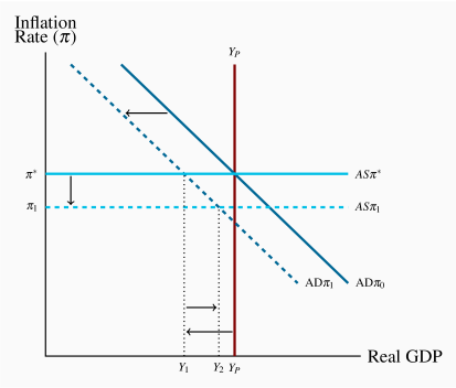
 to
to  creates a recessionary gap (Y1–YP). The increase in unemployment and reduction in output cuts the rate of increase in wage rates and prices to
  . Lower inflation leads the central bank to reduce its interest rate, supporting a move along
  to Y2.
In the short run, the fall in  creates a recessionary gap (Y1–YP). Since producers cannot cut costs per unit of output, they reduce employment and output to Y1 to cut total costs. Unemployment rates rise. At Y1 the goods market clears. It is a point on both the
  and
and  curves. Inflation has not fallen because of the short-run stickiness in wage rate increases and price increases.
 function the term
  defines this adjustment.
  shifts down to
  . As long as the central bank allows some flexibility in its policy interest rate, expenditure can increase along
  to Y2 and offset some of the output gap.
 curve. The output gap shrinks gradually but the inflation rate is below the central bank's target.
An inflationary gap results in the opposite process. Employment and output rise. Unemployment rates fall. Wage rate increases rise, inflation rises, and monetary policy reactions result in higher interest rates to reduce expenditure. In both cases, the eventual changes in wage rate agreements and rates of inflation together with the reaction of monetary policy to changes in inflation rates move the economy, over time, from short-run to long-run equilibrium. But the new equilibrium inflation rate would be higher than the Bank's target.
This adjustment process has important implications for the inflation targets set by monetary policy. It means prolonged changes in aggregate demand conditions require changes in the central bank's interest rate setting to defend the inflation target. It also means that, if the inflation target is cut, shifting the  curve to the left, the economy will go through a recession, and perhaps a prolonged recession, while money wage rate agreements are renegotiated and price setting practices adjust to reflect the new inflation target. The time required for this adjustment is linked in a very important way to the independence and the credibility of the central bank. Canadian experience in the 1990s provides an interesting example. Recessionary gaps were persistent after the Bank of Canada adopted an inflation target of 2 percent at a time when current inflation rates were about 5 percent.
An aggregate supply shock
Figure 11.7 shows the model's internal adjustment to unexpected shift in  . A sharp increase in crude oil and commodity prices, for example, enters the
  function as an increase in
  (
( ) in Equation 11.3. That pushes costs up and prices follow, increasing the inflation rate at least temporarily. Increases in indirect taxes like the HST or the taxes on alcohol and gasoline would have a similar effect. They increase the sellers' tax remittances to government, which sellers attempt to offset by increasing prices.
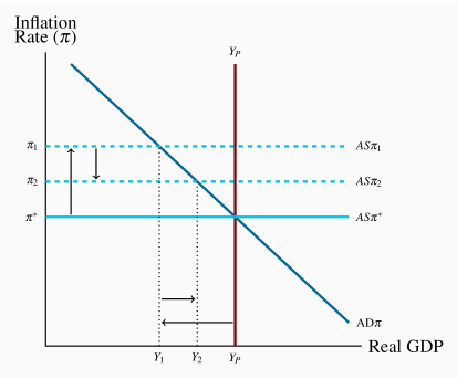
 increase
  as
as  shifts up to
  . Inflation is higher than the Bank's
  target and output falls, creating a recessionary gap. This is 'stagflation'. The central bank faces a dilemma. It cannot defend its inflation target without increasing the gap. Alternatively it can wait until
  falls back to
  .
.In Figure 11.7 the  curve shifts up to
  . The inflation rate is higher and output falls creating a recessionary gap. These are the economic conditions often described as 'stagflation'. They pose a dilemma for the central bank.
Inflation is higher than its official target rate but trying to bring inflation down by raising the policy interest setting would only make things worse by raising the unemployment rate. Alternatively, cutting the policy interest rate to reduce the recessionary gap would shift  to the right and validate the higher inflation rate. Doing nothing, on the assumption that the increase in commodity prices is a one-time jump, would mean living with inflation above the target and high unemployment until the rates of increase in wage rates and prices fall. Then
  would shift down to
  . The cost of waiting is the cumulative loss of employment and output during the adjustment process and the redistribution of income in favour of commodity producers if that is the source of the supply shift.
11.5 Monetary and fiscal policies
The inflation-output model sets clear roles for monetary and fiscal policies, at least in normal times. Monetary policy, which is embedded in the  curve, is aimed at an inflation control target using a short-term interest rate instrument. Within the structure of the model this monetary policy simultaneously moderates business cycle fluctuations in output and supports equilibrium output at potential output. Fiscal policy can be aimed at a government debt ratio target through budget balance control. The net tax rate in the government's budget provides automatic fiscal stabilization to moderate business cycle fluctuations.
Canadian monetary and fiscal policy followed this pattern from the early 1990s until the financial crisis of 2008. The Bank of Canada, in consultation with the Ministry of Finance has set inflation control targets for monetary policy since 1991. With the policy independence provided by a flexible exchange rate, the Bank uses the overnight interest rate as its policy instrument and intervenes in the market for overnight clearing balances. This keeps the overnight rate within the operating band it sets. An interest rate policy rule provides a useful description of the Bank's reactions to inflation rates that deviate from its control target.
Monetary policy
In practical terms central banks set their short-term interest rate instruments based on their inflation rate control target and their assessment of current and future economic conditions. This approach is described by a policy rule for setting the interest rate like that introduced in Chapter 10, namely:
 | (11.4) |
Adding a term for the output gap means the central bank looks at both the inflation rate and the state of the economy in making its interest rate setting decisions. In terms of the  model, the output gap is a predictor of the way the inflation rate will move if current conditions persist. In times of recession, for example, the output gap term in the policy rule calls for a cut in interest rates even if the inflation rate is still
  . This way the central bank pre-empts the fall in inflation that a recession would cause.
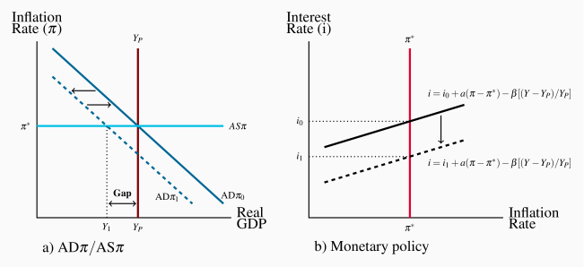
 in a) with the Bank's overnight rate set at i0. Then
  falls to
  as a global recession reduces exports. GDP falls to Y1 causing an output gap Y1–YP. The central bank reacts to the output gap with a cut in its overnight rate target to i1 in b), to provide stimulus and increase
  .
. . Lower
  creates a recessionary gap but does not immediately lower the inflation rate. The central bank sees the fall in
  as a lasting change in economic conditions that will reduce inflation below its inflation control target. It cuts its policy interest rate setting from i0 to i1 to increase
  , shifting
  to the right, and reduce the output gap and downward pressure the gap puts on the inflation rate.
 to
to  at least in part. You can read the full text of the press release at: http://goo.gl/W6UMg0.
Figure 11.9 shows that the Bank of Canada's setting for its overnight interest rate has been related to the output gap over the 1995–2017 period. The interest rate setting rule described by Equation 11.4 calls for the Bank to lower its overnight rate as the output gap (Y–YP)/YP is <0 and increase its rate when the output gap (Y–YP)/YP is >0. Figure 11.8 gives one example of how this works in theory. It is indeed the pattern of overnight rate settings we see in the data plotted in Figure 11.9.
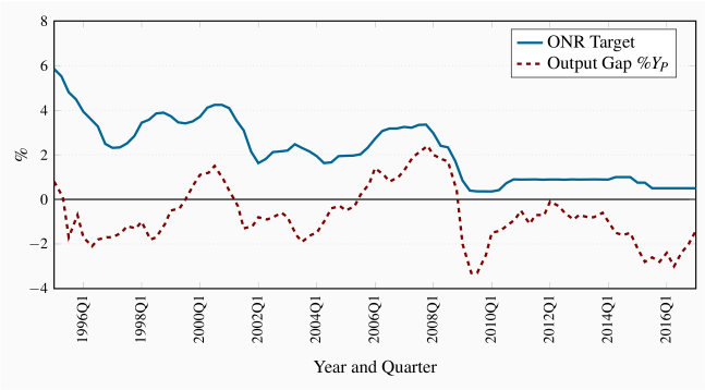
More recent examples of the Bank's reaction to an anticipated recession were the cuts in the overnight rate in 2015 following the drop in oil and commodity prices. This rate cut was intended to offset the negative effects of lower oil prices on the revenue, employment and investment expenditures of major oil and commodity producers. The economy was already working with a recessionary gap and that gap was growing in the first half of 2015.
 model, which explains changes in the inflation rate that follow from persistent output gaps. The
  function also provides for changes in the inflation rate as a result of other economic changes such as changes in the prices of raw materials or changes in indirect taxes. The Bank might change its overnight rate setting in response to these changes in inflation that are not driven by the output gaps.
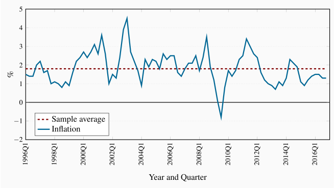
The data plotted in Figure 11.10 show the volatility of the annualized quarterly inflation rates but the average rate over the period is indeed 1.8 percent, just below the Bank's 2.0 percent target. Over the same period the economy went through both recessionary and inflationary gaps, with a small recessionary gap, -0.5 percent of YP, on average. If the period following the financial crisis of 2008 is excluded the average output gap from 1995 to 2008 is -0.2 percent with a range of -2.1 percent to +2.4 percent.
While success with inflation control did not eliminate the business cycle in real GDP and employment, economic performance was consistent with the argument of the  model. From 1995 to 2007 the inflation rate fluctuated around the 2 percent target and output was, on average, close to estimates of potential output.
The financial crisis of 2008 changed the economic fundamentals, the focus of monetary and fiscal policies, and the economic performance of the economy. This more recent experience is covered after a discussion of recent fiscal policy in terms of the  model.
Fiscal policy
Under normal conditions in the  model with a flexible foreign exchange rate, monetary policy dominates discretionary fiscal policy. Monetary policy sets the interest rate that will give the
  needed to get the inflation rate target at potential output. A change in discretionary fiscal policy would change the conditions on which the Bank's interest rate is set. To defend its inflation rate target the Bank would react, changing its interest rate setting to offset any new fiscal stimulus or restraint. Monetary policy aimed at inflation control deliberately crowds out the effect of fiscal policy on
  through the interest rate-exchange rate links in the monetary transmission mechanism.
For example, in 2006 and 2007 the Government of Canada cut the GST by a total of 2.0 percentage points. The Bank of Canada raised its overnight interest rate from 3.25 percent to 4.50 over the same time period. At the time the economy was also working at an inflationary gap. The increase in interest rates offset the fiscal stimulus from the GST cut by raising costs of current and future credit.
However, fiscal policy does have two important roles to play when the central bank successfully targets inflation and potential output:
Provide automatic fiscal stabilization; and
Control, and perhaps reduce, the ratio of the public debt to GDP.
Fiscal policy is implemented through the government's budget. The budget balance function provides the framework. Elaborating on the basic government budget of Chapter 7 to recognize the importance of the public debt gives:
 | (11.5) |
The term iPD is the interest paid on the government bonds, PD, issued in the past to finance budget deficits. G represents program spending. G+iPD is total government spending.
The fiscal policy instruments are:
The net tax rate, t, set in the budget plan, which will also be a component of,
The primary budget balance, PBB=tY–G, which excludes interest payments on the public debt.
The Department of Finance, Fiscal Reference Tables, 2016 (www.fin.gc.ca) report the Government of Canada paid interest (iPD) of $25.6 billion in the fiscal year 2015–16. That was an amount equal to 2.7 percent of its outstanding interest bearing debt and 8.6 percent of total government expense (G+iPD).
Government tax and expenditure programs linked to GDP provide automatic fiscal stabilization, as explained in Chapter 7. In addition, with a monetary policy consistent with equilibrium at potential output, discretionary fiscal policy can aim to control the public debt ratio (PD/Y) by managing the government's primary budget balance. This is the fiscal policy objective that has caused serious debates in both the US and Europe, and in the 2015 federal election campaign in Canada.
Public debt ratio (PD/Y): the ratio of government debt to GDP.
Primary budget balance (PBB=tY–G): the difference between net tax revenue at YP and government program expenditure. It excludes interest payments on the public debt.
Current interest payments on the public debt are the result of past issues of government bonds and the average of coupon rates on those bonds. This expenditure cannot be changed in the current budget but can be controlled going forward as current budget balances reduce or increase the public debt.
Automatic stabilization
Automatic fiscal stabilization comes from the net tax rate t in the budget function. This rate changes government revenues and transfers automatically when GDP changes. Cyclical changes in the government budget balance reduce the size of the expenditure multiplier and the size of the change in GDP caused by shifts in  conditions. The budget function:
 | (11.6) |
separates the cyclical component t(Y–YP) of the budget balance BB from the structural primary budget balance SPBB. The structural primary budget balance evaluates the government's fiscal program net of interest payments on the public debt at YP. The cyclical component is the effect of an output gap on the actual budget balance. The actual budget balance BB in Equation 11.6 has three components, the structural primary budget balance (SPBB), the cyclical component  and the interest payments on the public debt (iPD).
Setting the net tax rate that will provide automatic stabilization is a simple mechanical question but a difficult economic and political question. A higher net tax rate provides more stabilization. It involves the design of the tax system and transfer payment programs like employment insurance, social assistance programs and subsidy programs where revenues collected and expenditures made vary inversely to economic conditions. The types of taxes to be used and the bases to which those taxes are to be applied generate heated debates. The design and eligibility requirements for transfer benefits are also controversial. There are also strong differences of opinion over the economic impacts of different types and rates of taxes and transfers. These issues have been important to recent election campaigns in Canada and the US and will dominate ongoing US debates about budget deficits and public debt control.
We will leave the details of those debates to specialists in public finance and ask a question that is somewhat easier to answer. Have changes in the cyclical balance of the Canadian federal government budget provided automatic stabilization? To answer this question, Figure 11.11 plots the output gap and the cyclical budget balance over the 1995–2016 time period. These data show a pattern of cyclical budget deficits and surpluses that coincide with recessionary and inflationary gaps to provide automatic fiscal stabilization.
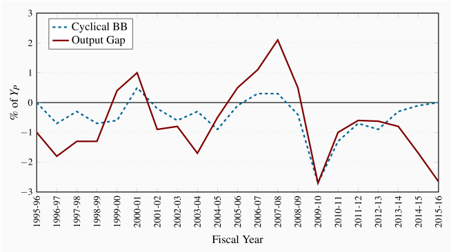
For most years in the period covered by Figure 11.11 the absolute magnitude of the cyclical budget balance is noticeably less than that of the output gap. That pattern changes after 2008 when expansionary fiscal policy, the 'Economic Action Plan' of 2009 was introduced to fight the recession that followed the 2008 financial crisis. Although this was clearly a discretionary policy change, the Department of Finance reported it in its Fiscal Reference Tables, 2011 as a component of the cyclical balance, excluding it from its structural budget balance estimates, and continues this practice with additional revisions in the Fiscal Reference Tables, 2016. This is an interesting treatment of this discretionary stimulus program that was extended into 2011 and 2014 and continued to feature prominently in government advertisements. As a result, the 'automatic stabilization' illustrated in Figure 11.11 is overstated in the 2009–2014 period and the reported structural budget balance is increased. Furthermore, in the 2013–2015 period the changes in cyclical budget balance reflect a shift to fiscal austerity driven by the Harper Conservative government's commitment to achieve a balanced budget, BB = 0, by 2015 even in a time of economic recession.
The Liberal government elected in 2015 offered an alternative approach. Government budget deficits for at least a few years based on infrastructure expenditure. The objective was to stimulate economic growth, reduce recessionary income gaps and unemployment by increasing aggregate demand and productivity. As economic conditions deteriorated as a result of falling oil and commodity prices budget deficits were larger than initially proposed, undermining the original time frame set for achieving a balanced budget. Control of the public debt ratio became the new constraint on fiscal stimulus and the budget deficit.
Setting a target for the public debt ratio defines both the size of the primary budget balance and the budget deficit the government can run. It also defines the scale of the fiscal expansion or austerity the government has to work with.
Controlling the debt ratio
The public debt ratio is usually defined as the outstanding public debt as a percentage of annual nominal GDP. Explaining the budget balances required to control and reduce the public debt ratio is a bit more complicated. The annual change in the outstanding public debt, PD, is equal to the annual budget deficit or surplus,  . The change in the debt ratio, PD/Y from one year to the next is determined by two conditions namely:
The percentage change in the debt,
 , which is the change in the numerator of the ratio and
The percentage change in GDP,
 , which is the change in the denominator of the ratio.
Recall that the government's budget balance function is:
BB=tY–G–iPDWhere the net tax rate t, and government program expenditure G are set in annual budgets. The third component, iPD, is determined outstanding public debt and the average interest rate on that debt. As a result it is only the primary budget balance (PBB = tY – G) that can be changed in annual budgets.
Furthermore, if the primary budget is balanced, (PBB = tY – G = 0) interest payments on the outstanding debt will still increase the debt by iPD. This increase in the public debt will increase the debt ratio unless there is an offsetting increase in GDP. As a result the difference between the interest rate, i, that increases the debt, the growth rate of GDP, g, and the current debt ratio, PD/Y, determine the primary budget balance relative to GDP, PBB/Y, required to keep the debt ratio constant, namely:
 | (11.7) |
Table 11.1 uses Equation 11.7 to provide a numerical example of a change in the Government of Canada's debt ratio based on a small sample of recent data from the Department of Finances Fiscal Reference Tables 2016. Columns (2), (3) and (4) show the interest rate, growth rate and public debt ratio used to estimate the primary budget balance required to stabilize the public debt ratio at its fiscal year end value of 31.3 percent.
Based on these conditions, with the interest rate on the public debt, i = 3.2 percent, less than the growth rate in nominal GDP, g = 4.5 percent, the debt ratio would have been constant even with a small primary budget deficit, PBB < 0, of about 0.04 percent. As it turned out, the government's actual primary budget surplus reduced the debt ratio from 31.3 percent in 2013–14 to 29.6 percent in 2014–15. Strong growth in nominal GDP was important for this outcome.
| (1) | (2) | (3) | (4) | (5) | (6) | (7) |
| Time | Interest rate | Growth rate | Public debt | PBB/Y required | Observed | Observed |
| Period | on public debt | of nominal GDP | ratio | for  | PBB/Y |  |
| i | g | PD/Y | ||||
| 2013–2014 | 0.032 | 0.045 | 0.313 | -0.004 | 0.012 | -0.016 |
The current Government of Canada is not the first to identify the debt ratio as a constraint on fiscal policy. In 1994 the Government of Canada announced A New Framework for Economic Policy that focused fiscal policy on deficit control and debt ratio reduction: goo.gl/GZKyxP. It set an initial budget deficit target of 3 percent of GDP as the first step in a fiscal policy program aimed at achieving first a balanced budget and then a surplus to reduce the federal government debt as a percentage of GDP. This was followed in 2004 by a target: Reducing the debt-to-GDP ratio to 25 percent within 10 years. The government then managed the budget balance through a combination of taxation and expenditure programs to pursue this debt ratio target.
When this policy announcement was made the public debt stood at 68 percent of GDP. The primary budget balance was in deficit and interest payments on the public debt absorbed about 35 percent of government revenue. In the years that followed, the public debt ratio declined steadily to a low 29 percent in 2008–09. Interest payments on the debt fell to less than 13 percent of revenue. Fiscal policy was on track to meet the debt ratio target of 25 percent set in the 2004 Budget. Significant primary surpluses were the major fiscal contributor to this decline in the ratio. The fiscal stimulus introduced in 2009 reversed this pattern, creating budget deficits and raising the net public debt by 30 percent between 2009 and 2014.
Canadian success with debt ratio control and reduction from 1995 until 2009 has been cited as an example for countries currently facing very high debt ratios. But it may not fit with current economic conditions in those countries. Canada's fiscal adjustment was made easier by a substantial easing of monetary conditions in terms of both interest rates and exchange rates and strong growth in the US economy, which all supported a large increase in exports and growth in Canadian GDP. This economic environment is not available to the countries that now face a debt crisis.
Even with favourable conditions, the Canadian adjustment was costly. There was a cumulative loss of output from an output gap that lasted from 1995 to 1999 that was at times as large as 2 percent of YP. Unemployment rates reached 9 percent and low rates of capacity utilization in industry reduced profitability and investment in new capacity and technology.
These and the negative fiscal effects of the earlier monetary restraint following the shift to inflation targeting are now sunk costs. In the years that followed monetary and fiscal policies worked to deliver stable inflation and declining public debt ratios until the crisis and recession of 2008–09.
11.6 Recession, disinflation and deflation
The financial crisis of 2008 and the recession that followed uncovered the limitations of monetary policy and renewed the case for fiscal stimulation. The assignment of monetary policy to an inflation target at YP and fiscal policy to debt ratio control did not work in the new economic conditions. Moreover, the depth of the recession and the collapse of the U.S. banking and financial sectors led to disinflation and raised fears of deflation as a result of rising real interest rates and output gaps. The Great Depression of the 1930s was an historical example. The Japanese experience starting in the 1990s with zero interest rates and a continuing slump was another. Stephan Poloz, the Governor of the Bank of Canada has at times worried out loud about the risks of deflation in Canada and discussed concerns briefly in an earlier speech on monetary policy. The full text of that speech is available at:
http://www.bankofcanada.ca/2013/12/monetary-policy-as-risk-management/
Although the risk of deflation has receded the issues raised by disinflation remain at least as long as central banks have reached the zero lower bound and cannot provide monetary stimulus through interest rate cuts. A rethinking of macroeconomic policy was necessary.
Disinflation: a persistent fall in the inflation rate.
Deflation: a persistent fall in the general price level.
Some of the issues involved can be explained with the basic  model. In Figure 11.12 a financial crisis shifts
  by undermining the interest rate-expenditure link in the monetary transmission mechanism. Financial risk and uncertainty increase and demands for liquidity increase. Banks are reluctant to lend and businesses are reluctant to borrow. The
  curve shifts left and pivots to show the reduction in financing and the fall in the interest sensitivity of expenditure. Equilibrium shifts to
  with a recessionary gap.
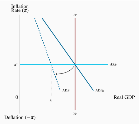
 falls but central bank interest rate cuts cannot offset the fall in
  . At zero lower bound deflation raises real interest rate and the output gap continues to grow.
The recessionary gap triggers two reactions. The inflation rate falls and the central bank cuts its interest rate to offset the fall in inflation and output. But the steeper  function reflects the disruption to financial markets. Nominal interest rate cuts have limited the effects on expenditure. To prevent a rise in the real interest rate
  the Bank must cut its nominal policy rate by more than the fall in inflation.
But the central bank cannot lower its rate below zero – it hits the lower bound. If the output gap persists and pushes disinflation into deflation, rising real interest rates cut expenditure and increase the gap. The  function would be kinked backward at i=0 to capture these negative effects of disinflation and deflation. Falling inflation rates reduce aggregate expenditure and aggregate demand along the
  curve.
Fortunately economic conditions did not deteriorate badly enough to trigger deflation:
"It appears today that the world will likely avoid a major deflation and thus avoid the deadly interaction of larger and larger deflation, higher and higher real interest rates and larger and larger output gaps."
Blanchard, O. et al. (2010). Rethinking Macroeconomic Policy. IMF Staff Position Note, SPN/10/03
Nevertheless, faced with the financial crisis and recession, major industrial countries shifted their policy programs. Cutting interest rates to defend inflation targets was the first policy initiative. The Bank of Canada cut its target overnight interest rate from 4.25 percent in late 2007 to a record low 0.25 percent in early 2009 and held the rate at that level until mid-2010. In the US the Federal Reserve cut its federal funds rate, the policy rate that corresponds to the Bank of Canada's overnight rate, from 5.25 percent in late 2007 to 0.0 percent in late 2008. It is still at that rate today in late 2014. These interest rate cuts reduced policy rates to the zero lower bound and exhausted the potential for monetary stimulus with that policy instrument.
Monetary policy in the US turned then to instruments used before it adopted interest rate setting to get an inflation target. The first was increased "moral suasion," an increase in communications with financial market participants, including conditional statements about the future path of policy rates, to emphasize the central bank's longer-term support for markets and its actions to promote stability. More directly the banks were urged to maintain their lending operations. The second was "quantitative easing," and in the case of the US, an even more extensive "credit easing." "Quantitative easing" extends the use of open market operations described above. The central bank purchases a broader range of financial assets to expand its balance sheet to increase substantially the monetary base and cash positions of the banks. In other words, the objective is to increase the quantity of cash reserves in the banking system directly.
Quantitative easing: a central bank purchase of financial assets to increase its asset holdings and the monetary base.
Credit easing: the management of the central bank's assets designed to support lending in specific financial markets.
Open market operations usually involve central bank purchases of short-term government bonds. The US Federal Reserve went beyond this, introducing three sets of policy tools:
lending to financial institutions,
providing liquidity directly to other key credit markets by buying highly rated commercial paper, and
buying longer-term securities, including mortgage backed securities.
Using these tools increases the size of the central bank's balance sheet and changes the structure of central bank asset holdings. Quantitative easing is measured by the impact on the quantity of bank reserves. Credit easing is measured by the wider variety of loans and securities the central bank willingly holds on its balance sheet. A purchase of these assets puts cash directly into specific markets rather than feeding it through banks and bank lending. Both are intended to increase lending to businesses and households in times when very low, near zero, interest rates alone are not working.
The effect of three rounds of quantitative easing by the US Federal Reserve has been to raise the monetary base in the US from about $800 billion in to $2.62 trillion in October 2012. While this monetary stimulus has not offset the full effects of the 2008-09 recession, it is credited with avoiding a US deflation. A version of this policy action was used in Japan earlier in the decade after the Bank of Japan had lowered its borrowing rate to zero and wanted to provide further economic stimulus. In terms of the  model the intent was to support demand and shift the
  curve to the right or least avoid deflation if recessionary gaps persisted.
The Bank of Canada also developed plans for quantitative easing that were not used as economic conditions improved more quickly here than in some other countries. You can see the Bank's explanation of these policies in its Monetary Policy Report, April 2009 pp. 24-28, at http://www.bankofcanada.ca/wp-content/uploads/2010/03/mpr230409.pdf.
These monetary policies were supported by discretionary fiscal policies. With interest rates a zero, crowding out was not a concern and increased  was the objective. The earlier focus on deficit and debt ratio control was set aside to provide aggregate demand stimulus. In Canada the federal government's 'Action Plan' included direct support for infrastructure projects and tax incentives for certain household expenditures. In terms of budget data the federal government structural budget shifted from a surplus of $3.8 billion in fiscal 2007–08 to a deficit of $10.6 billion in 2009–10. But as noted earlier, the 'Action Plan' stimulus was treated as a 'cyclical' budget component. Thus the change in the actual federal budget balance from a surplus of $9.6 billion in fiscal 2007–08 to a deficit of $55.6 billion in fiscal 2009–10 is probably a better measure of the fiscal stimulus that addressed the recession. However, this stimulus was relatively short lived as the government returned to its earlier deficit and debt control focus and left monetary policy to provide sustained support for economic recovery. The monetary/fiscal policy mix remained that way in mid-2015 leading up to the federal election in the fall of that year.
The new federal government led by Prime Minister Justin Trudeau shifted from a balanced budget fiscal plan to budgets designed to promote economic growth based on major infrastructure investment and modest tax cuts financed by modest budget deficits. This fiscal stimulus together with continued monetary stimulus from the Bank of Canada shifted policy mix from fiscal austerity/monetary stimulus to fiscal and monetary stimulus combined. Evaluating the effectiveness of this mix lies in the future.
 curve
curve The  curve is based on:
An AE function that includes the effect of interest rates on expenditures, and
Central bank monetary policy that sets interest rates to defend an inflation rate target.
 | (1) |
 , the marginal propensity to spend. Using the equilibrium expenditure condition
  gives:

 | (2) |
 | (3) |
 is the Bank's inflation rate target and
  is the actual inflation rate. With
  the central bank's response to a change in the inflation rate changes the nominal interest rate enough to change the real interest rate. The monetary policy objective is to keep inflation at the target value
  .
Substituting the interest rate determined by monetary policy in 11.10 into the equilibrium expenditure condition 11.9 gives an aggregate demand curve that includes the inflation rate:
 | (4) |
 to distinguish it from the traditional P, Y aggregate demand curve.
  is the relationship between real output and inflation.
A numerical example illustrates this AD
 curve. Suppose
 and the central bank has an inflation target
  percent. The bank estimates that a real interest rate of 2.0 percent is needed for equilibrium at potential output. It sets the nominal interest rate
  and reacts to transitory departures from its inflation target according to the policy rule:
 Then by substitution,
 |  |
 |  |
 giving:
 | (5) |
 defines a negative relationship between the inflation rate and equilibrium real GDP.
When the inflation rate is equal to the monetary policy target of 1 percent (
 ), the equilibrium level of real GDP and demand is 340. If the inflation rate were to rise to 1.5 percent, which exceeds the target by 0.5 percent, the Bank's reaction would be to raise the interest rate by
  percent. This would lower aggregate expenditure by
  and equilibrium real GDP by
  to 325, moving up along the
  curve. A fall in inflation from the target would bring the opposite reaction. This scenario is depicted in Figure 11.13.
 curve
curve 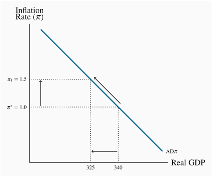
Next
This chapter provides the basic model for the analysis of macroeconomic performance and policy that integrates the design, instruments and objectives of modern monetary and fiscal policies. Inflation, deflation, public debt ratios and business cycles are explained. But two issues remain. One is international macroeconomics and the importance of exchange rate policy for the effectiveness of monetary and fiscal policies. The second is economic growth, growth theory and growth accounting. These are covered in the next two chapters.
Key Concepts
The AD curve describes the relationship between equilibrium real GDP and the inflation rate.
Monetary policy that sets an inflation rate target and uses the short-run interest rate as a policy instrument is integral to the AD curve.
The production function  determines the output of goods and services.
In the long run, labour market equilibrium determines the equilibrium level of employment and potential output YP.
In the short run, employment and output fluctuate in response to changing economic conditions. However, there is no trade-off between inflation rates and output.
The short run AS function describes the lagged adjustment to the inflation rate in reaction to output gaps.
The AS function is based on the price setting decisions of producers in imperfectly competitive markets.
The equilibrium inflation rate is the inflation control target set by the central bank.
Business cycles in output and employment caused by persistent AD and/or AS
 shifts create output gaps.
Persistent output gaps lead to an internal adjustment based on changes in the rate of increase in money wage rates and changes in the rate of inflation.
A monetary policy rule describes the central bank's setting of its interest rate policy instrument as reactions to inflation rates that differ from its inflation control target and to output gaps.
Fiscal policy controls government budget balances to control or reduce the size of the public debt ratio.
The primary budget balance is the fiscal policy instrument.
The arithmetic of changes in the public debt ratio links the change in the debt ratio to the primary budget balance and the difference between the interest rate on the debt and the growth rate of GDP.
Over the 1995–2008 period Canadian monetary and fiscal policies effectively controlled the Canadian inflation rate and reduced the federal government debt ratio.
The financial crisis of 2008 and the recession that followed in 2008–09 demonstrated the limits of monetary policies based on interest rates and fiscal policies focused on debt ratio control. In Canada, a combination of monetary and fiscal stimulus reduced the fall in output and employment. In other countries, a broader set of monetary policy instruments and fiscal austerity have yet to solve employment and public debt issues.
Exercises for Chapter 11
Use a diagram to illustrate an economy at the equilibrium inflation rate. In this diagram, show how a permanent increase in exports would affect the equilibrium inflation rate and the equilibrium level of GDP if the central bank did not react and change its monetary policy.
Suppose the central bank reacted to defend its inflation target from the effect of the increase in exports in Exercise 11.1. Use an  diagram to show the change in the equilibrium interest rate setting and real GDP you would observe.
Suppose opportunities for investing in high tech applications boost aggregate demand in the short run, and aggregate supply in the long run. Using  and
and  curves with equilibrium at potential output, show why output might rise in the long run without much of an increase in inflation.
Suppose a new round of labour negotiations results in a higher average rate of increase in money wage rates for the next three years. Illustrate and explain how this would affect short-run aggregate supply conditions and the  curve.
Draw an aggregate supply and demand curve diagram to show an economy in short-run equilibrium at potential output. Suppose a wide-spread recession reduces incomes in foreign countries, leading to reduced demand for exports. Illustrate and explain how this would affect the short-run equilibrium Y and  in your diagram.
Suppose central banks have reduced their policy interest rates to the lower bound to fight a deep and prolonged recession. Use a diagram to show how either a reduction in the inflation rate, or deflation, would change the slope of the  curve. Would cuts in nominal money wage rates and further reductions in the inflation rate reduce the recessionary gap when the central bank is constrained by the lower bound on its interest rate?
In the two years before 2008 the Canadian federal government reduced the GST from 7 percent to 5 percent. Use an  diagram to illustrate and explain the effects of this tax change on equilibrium output and inflation. If the economy was in equilibrium at YP and the target inflation rate
  before the tax cut, what monetary policy action, if any, would the central bank make to maintain those equilibrium conditions after the tax cut? What short-run net benefit, if any, would households and businesses realize as a result of the cut in the GST?
Define the 'public debt' and explain why and how it might increase from one year to the next.
Would it be possible for the ratio of the public debt to GDP (PD/Y) to fall even if the government's primary budget is in deficit? Explain your answer.
Would it be possible for the ratio of public debt to GDP (PD/Y) to rise even if the government's primary budget balance is in surplus? Explain your answer.
Optional: Suppose the central bank's monetary policy sets the interest rate according to the function:

and aggregate expenditure is the sum of:
| C | =200+0.75Y |
| I | =85–2i |
| G | =100 |
| X–IM | =50–0.15Y–3i |
What is the equation for the
 curve?
Plot the
 curve in a diagram, not necessarily to scale, that shows the horizontal intercept and slope of the curve.
Optional: If careful research estimates potential output YP at 1,000, and the  function is as derived in Exercise 11.11, what is the equilibrium inflation rate? What interest rate must the central bank set to defend its inflation target?


