In this chapter we will explore:
| 2.1 | Data analysis
|
| 2.2 | Data, theory and economic models
|
| 2.3 | Ethics, efficiency and beliefs
|
Economists, like other scientists and social scientists, observe and analyze
behaviour and events. Economists are concerned primarily with the economic
causes and consequences of what they observe. They want to understand an
extensive range of human experience, including: money, government finances,
industrial production, household consumption, inequality in income
distribution, war, monopoly power, health, professional and amateur sports,
pollution, marriage, the arts, and much more.
Economists approach these issues using theories and models. To present,
explain, illustrate and evaluate their theories and models they have
developed a set of techniques or tools. These involve verbal descriptions
and explanations, diagrams, algebraic equations, data tables and charts and
statistical tests of economic relationships.
This chapter covers some of these basic techniques of analysis.
2.1 Data analysis
The analysis of behaviour necessarily involves data. Data may serve to
validate or contradict a theory. Data analysis, even without being motivated
by economic theory, frequently displays patterns of behaviour that merit
examination. The terms variables and data are related. Variables are measures that can take on different magnitudes.
The interest rate on a student loan, for example, is a variable with a
certain value at a point in time but perhaps a different value at an earlier
or later date. Economic theories and models explain the causal relationships
between variables. In contrast, Data are the recorded values
of variables. Sets of data provide specific values for the variables we want
to study and analyze. Knowing that gross domestic product (a variable)
declined in 2009 is just a partial description of events. If the data
indicate that it decreased by exactly 3%, we know a great deal more – the decline was large.
Variables: measures that can take on different values.
Data: recorded values of variables.
Sets of data help us to test our models or theories, but first we need to
pay attention to the economic logic involved in observations and modelling.
For example, if sunspots or baggy pants were found to be correlated with
economic expansion, would we consider these events a coincidence or a key to
understanding economic growth? The observation is based on facts or data, but
it need not have any economic content. The economist's task is to
distinguish between coincidence and economic causation. Merely because
variables are associated or correlated does not mean that one causes the
other.
While the more frequent wearing of loose clothing in the past may have been
associated with economic growth because they both occurred at the same time
(correlation), one could not argue on a logical basis that this behaviour
causes good economic times. Therefore, the past association of these
variables should be considered as no more than a coincidence. Once specified
on the basis of economic logic, a model must be tested to determine its
usefulness in explaining observed economic events.
Table 2.1 House prices and price indexes
|
Year | House | Percentage | Percentage | Real | Index for | 5-year |
|
| prices in | change in  | change in | percentage | price of | mortgage |
|
| dollars | | consumer | change | housing | rate |
|
| () | | prices | in | | |
|
2001 | 350,000 | | | | 100 | 7.75 |
|
2002 | 360,000 | | | | 102.9 | 6.85 |
|
2003 | 395,000 | 35,000/360,000=9.7% | 3% | 6.7% | 112.9 | 6.6 |
|
2004 | 434,000 | | | | 124.0 | 5.8 |
|
2005 | 477,000 | | | | 136.3 | 6.1 |
|
2006 | 580,000 | | | | 165.7 | 6.3 |
|
2007 | 630,000 | | | | 180.0 | 6.65 |
|
2008 | 710,000 | | | | 202.9 | 7.3 |
|
2009 | 605,000 | -105,000/710,000=-14.8% | 1.6% | -16.4% | 172.9 | 5.8 |
|
2010 | 740,000 | | | | 211.4 | 5.4 |
|
2011 | 800,000 | | | | 228.6 | 5.2 |
Note: Data on changes in consumer prices come from Statistics Canada, CANSIM series V41692930; data on house prices are for N. Vancouver from
Royal Le Page; data on mortgage rates from
http://www.ratehub.ca. Index for house prices obtained by scaling each entry in column 2 by 100/350,000. The real percentage change in the price of housing is: The percentage change in the price of housing minus the percentage change in consumer prices.
Data types
Data come in several forms. One form is time-series, which
reflects a set of measurements made in sequence at different points in time.
The first column in Table 2.1 reports the values for
house prices in North Vancouver for the first quarter of each year, between
2001 and 2011. Evidently this is a time series. Annual data report one
observation per year. We could, alternatively, have presented the data in
monthly, weekly, or even daily form. The frequency we use depends on the
purpose: If we are interested in the longer-term trend in house prices, then
the annual form suffices. In contrast, financial economists, who study the
behaviour of stock prices, might not be content with daily or even hourly
prices; they may need prices minute-by-minute. Such data are called high-frequency data, whereas annual data are low-frequency data.
Table 2.2 Unemployment rates, Canada and Provinces, monthly 2012, seasonally adjusted
|
| Jan | Feb | Mar | Apr | May | Jun |
|
CANADA | 7.6 | 7.4 | 7.2 | 7.3 | 7.3 | 7.2 |
|
NFLD | 13.5 | 12.9 | 13.0 | 12.3 | 12.0 | 13.0 |
|
PEI | 12.2 | 10.5 | 11.3 | 11.0 | 11.3 | 11.3 |
|
NS | 8.4 | 8.2 | 8.3 | 9.0 | 9.2 | 9.6 |
|
NB | 9.5 | 10.1 | 12.2 | 9.8 | 9.4 | 9.5 |
|
QUE | 8.4 | 8.4 | 7.9 | 8.0 | 7.8 | 7.7 |
|
ONT | 8.1 | 7.6 | 7.4 | 7.8 | 7.8 | 7.8 |
|
MAN | 5.4 | 5.6 | 5.3 | 5.3 | 5.1 | 5.2 |
|
SASK | 5.0 | 5.0 | 4.8 | 4.9 | 4.5 | 4.9 |
|
ALTA | 4.9 | 5.0 | 5.3 | 4.9 | 4.5 | 4.6 |
|
BC | 6.9 | 6.9 | 7.0 | 6.2 | 7.4 | 6.6 |
Source: Statistics Canada CANSIM Table 282-0087.
Time-series: a set of measurements made sequentially at different points in time.
High (low) frequency data: series with short (long) intervals between observations.
In contrast to time-series data, cross-section data record the
values of different variables at a point in time. Table 2.2
contains a cross-section of unemployment rates for
Canada and Canadian provinces economies. For January 2012 we have a snapshot
of the provincial economies at that point in time, likewise for the months
until June. This table therefore contains repeated cross-sections.
When the unit of observation is the same over time such repeated cross
sections are called longitudinal data. For example, a health survey that
followed and interviewed the same individuals over time would yield
longitudinal data. If the individuals differ each time the survey is
conducted, the data are repeated cross sections.
Longitudinal data therefore follow the same units of observation through time.
Cross-section data: values for different variables recorded at a point in time.
Repeated cross-section data: cross-section data recorded at regular or irregular intervals.
Longitudinal data: follow the same units of observation through time.
Graphing the data
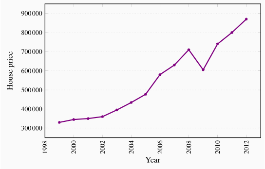
Data can be presented in graphical as well as tabular form. Figure 2.1
plots the house price data from the second column of Table 2.1. Each
asterisk in the figure represents a price value and a corresponding time
period. The horizontal axis reflects time, the vertical axis price in
dollars. The graphical presentation of data simply provides a visual rather
than numeric perspective. It is immediately evident that house prices
increased consistently during this 11-year period, with a single downward
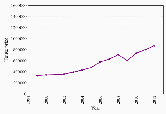
'correction' in 2009. We have plotted the data a second time in Figure 2.2 to
illustrate the need to read graphs carefully. The greater apparent
slope in Figure 2.1 might easily be interpreted to
mean that prices increased more steeply than suggested in Figure 2.2.
But a careful reading of the axes reveals that this
is not so; using different scales when plotting data or constructing
diagrams can mislead the unaware viewer.
Percentage changes
The use of percentages makes the analysis of data particularly simple.
Suppose we wanted to compare the prices of New York luxury condominiums with
the prices of homes in rural Mississippi. In the latter case, a change in
average prices of $10,000 might be considered enormous, whereas a change of
one million dollars in New York might be pretty normal – because the
average price in New York is so much higher than in Mississippi. To make
comparisons between the two markets, we can use the concept of a percentage change. This is defined as the change in the value
of the variable, relative to its initial value, multiplied by 100.
Percentage change .
.
The third column of Table 2.1 contains the values of the percentage change
in house prices for two pairs of years. Between 2002 and 2003 the price
change was $35,000. Relative to the price in the first of these two years
this change was the fraction 35,000/395,000=0.097. If we multiply this
fraction by 100 we obtain a percentage price change of 9.7%. Evidently we
could calculate the percentage price changes for all pairs of years. A
second price change is calculated for the 2008-2009 pair of years. Here
price declined and the result is thus a negative percentage change.
Consumer prices
Most variables in economics are averages of the components that go into
them. When variables are denominated in dollar terms it is important to be
able to interpret them correctly. While the house price series above
indicates a strong pattern of price increases, it is vital to know if the
price of housing increased more or less rapidly that other prices in the
economy. If all prices in the economy were increasing in line with house
prices there would be no special information in the house price series.
However, if house prices increased more rapidly than prices in general, then
the data indicate that something special took place in the housing market
during the decade in question. To determine an answer to this we need to
know the degree to which the general price level changed each year.
Statistics Canada regularly surveys the price of virtually every
product produced in the economy. One such survey records the prices of goods
and services purchased by consumers. Statistics Canada then computes an
average price level for all of these goods combined for each time period the
survey is carried out (monthly). Once Statistics Canada has computed the
average consumer price, it can compute the change in the price level from
one period to the next. In Table 2.1 two such values are entered in the
following data column: Consumer prices increased by 3% between 2002 and
2003, and by 1.6% between 2008 and 2009. These percentage changes in the
general price level represent inflation if prices increase,
and deflation if prices decline.
In this market it is clear that housing price changes were substantially
larger than the changes in consumer prices for these two pairs of years. The
next column provides information on the difference between the house price
changes and changes in the general consumer price level, in percentage
terms. This is (approximately) the change in the relative price of housing,
or what economists call the real price of housing. It is
obtained by subtracting the rate of change in the general price index from
the rate of change in the variable of interest.
Consumer price index: the average price level for consumer goods and services.
Inflation (deflation) rate: the annual percentage increase (decrease) in the level of consumer prices.
Real price: the actual price adjusted by the general (consumer) price level in the economy.
Index numbers
Statistics Canada and other statistical agencies frequently present data in index number form. An index number provides an easy
way to read the data. For example, suppose we wanted to compute the
percentage change in the price of housing between 2001 and 2007. We could do
this by entering the two data points in a spreadsheet or calculator and do
the computation. But suppose the prices were entered in another form. In
particular, by dividing each price value by the first year value and
multiplying the result by 100 we obtain a series of prices that are all
relative to the initial year – which we call the base year. The resulting
series in column 6 of Table 2.1 is an index of house price values. Each entry is the
corresponding value in column 2, divided by the first entry in column 2. For example, the value 124.0 in row 4 is obtained as  . The key
characteristics of indexes are that they are not dependent upon the
units of measurement of the data in question, and they are interpretable
easily with reference to a given base value. To illustrate, suppose we wish
to know how prices behaved between 2001 and 2007. The index number column
immediately tells us that prices increased by 80%, because relative to
2001, the 2007 value is 80% higher.
. The key
characteristics of indexes are that they are not dependent upon the
units of measurement of the data in question, and they are interpretable
easily with reference to a given base value. To illustrate, suppose we wish
to know how prices behaved between 2001 and 2007. The index number column
immediately tells us that prices increased by 80%, because relative to
2001, the 2007 value is 80% higher.
Index number: value for a variable, or an average of a set of variables, expressed relative to a given base value.
Furthermore, index numbers enable us to make comparisons with the
price patterns for other goods much more easily. If we had constructed a
price index for automobiles, which also had a base value of 100 in 2001, we
could make immediate comparisons without having to compare one set of
numbers defined in thousands of dollars with another defined in hundreds of
thousands of dollars. In short, index numbers simplify the interpretation of
data.
2.2 Data, theory and economic models
Let us now investigate the interplay between economic theories on the one
hand and data on the other. We will develop two examples. The first will be
based upon the data on house prices, the second upon a new data set.
House prices – theory
Remember from Chapter 1 that a theory is a logical argument regarding economic
relationships. A theory of house prices would propose that the price of
housing depends upon a number of elements in the economy. In particular, if
borrowing costs are low then buyers are able to afford the interest costs on
larger borrowings. This in turn might mean they are willing to pay higher
prices. Conversely, if borrowing rates are higher. Consequently, the
borrowing rate, or mortgage rate, is a variable for an economic model of
house prices. A second variable might be available space for development: If
space in a given metropolitan area is tight then the land value will reflect
this, and consequently the higher land price should be reflected in higher
house prices. A third variable would be the business climate: If there is a
high volume of high-value business transacted in a given area then buildings
will be more in demand, and that in turn should be reflected in higher
prices. For example, both business and residential properties are more
highly priced in San Francisco and New York than in Moncton, New Brunswick. A
fourth variable might be environmental attractiveness: Vancouver may be more
enticing than other towns in Canada. A fifth variable might be
the climate.
House prices – evidence
These and other variables could form the basis of a theory of house
prices. A model of house prices, as explained in Chapter 1, focuses upon
what we would consider to be the most important subset of these variables.
In the limit, we could have an extremely simple model that specified a
dependence between the price of housing and the mortgage rate alone. To test
such a simple model we need data on house prices and mortgage rates. The
final column of Table 2.1 contains data on the 5-year fixed-rate mortgage
for the period in question. Since our simple model proposes that prices
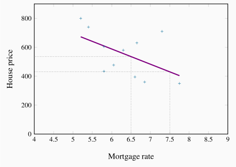
depend (primarily) upon mortgage rates, in Figure 2.3 we plot the
house price series on the vertical axis, and the mortgage rate on the
horizontal axis, for each year from 2001 to 2011. As before, each point (shown as a '+')
represents a pair of price and mortgage rate values.
The resulting plot (called a scatter diagram) suggests that there is a
negative relationship between these two variables. That is, higher prices
are correlated with lower mortgage rates. Such a correlation is consistent
with our theory of house prices, and so we might conclude that changes in
mortgage rates cause changes in house prices. Or at least the data
suggest that we should not reject the idea that such causation is in the
data.
House prices – inference
To summarize the relationship between these variables, the pattern suggests
that a straight line through the scatter plot would provide a reasonably
good description of the relationship between these variables. Obviously it
is important to define the most appropriate line – one that 'fits' the data
well. The line we have
drawn through the data points is informative, because it relates the two
variables in a quantitative manner. It is called a regression line. It predicts that, on average, if the mortgage rate
increases, the price of housing will respond in the downward direction. This
particular line states that a one point change in the mortgage rate will
move prices in the opposing direction by $105,000. This is easily verified
by considering the dollar value corresponding to say a mortgage value of
6.5, and then the value corresponding to a mortgage value of 7.5. Projecting
vertically to the regression line from each of these points on the
horizontal axis, and from there across to the vertical axis will produce a
change in price of $105,000.
Note that the line is not at all a 'perfect' fit. For example, the mortgage
rate declined between 2008 and 2009, but the price declined also – contrary
to our theory. The model is not a perfect predictor; it states that on average a change in the magnitude of the x-axis variable leads to a
change of a specific amount in the magnitude of the y-axis variable.
In this instance the slope of the line is given by -105,000/1, which is the
vertical distance divided by the corresponding horizontal distance. Since
the line is straight, this slope is unchanging.
Regression line: representation of the average relationship between two variables in a scatter diagram.
Road fatalities – theory, evidence and inference
Table 2.3 contains data on annual road fatalities per 100,000 drivers for
various age groups. In the background, we have a theory, proposing
that driver fatalities depend upon the age of the driver, the quality of
roads and signage, speed limits, the age of the automobile stock and perhaps
some other variables. Our model focuses upon a subset of these variables,
and in order to present the example in graphical terms we specify fatalities
as being dependent upon a single variable – age of driver.
Table 2.3 Non-linearity: Driver fatality rates Canada, 2009
|
Age of driver | Fatality rate |
|
| per 100,000 drivers |
|
20-24 | 9.8 |
|
25-34 | 4.4 |
|
35-44 | 2.7 |
|
45-54 | 2.4 |
|
55-64 | 1.9 |
|
65+ | 2.9 |
Source: Transport Canada, Canadian motor vehicle traffic collision statistics, 2009.
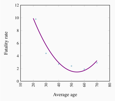
The scatter diagram is presented in Figure 2.4. Two aspects of this plot
stand out. First, there is an exceedingly steep decline in the fatality rate
when we go from the youngest age group to the next two age groups. The
decline in fatalities between the youngest and second youngest groups is
5.4 points, and between the second and third age groups
is 1.7 points. The decline between the third and fourth groups is minimal - just 0.3 points. Hence, behaviour is not the same
throughout the age distribution. Second, we notice that fatalities increase
for the oldest age group, perhaps indicating that the oldest drivers are not
as good as middle-aged drivers.
These two features suggest that the relationship between fatalities and age
differs across the age spectrum. Accordingly, a straight line would not be an
accurate way of representing the behaviours in these data. A straight line
through the plot implies that a given change in age should have a similar
impact on fatalities, no matter the age group. Accordingly we have an
example of a non-linear relationship. Such a non-linear
relationship might be represented by the curve going through the plot.
Clearly the slope of this line varies as we move from one age category to
another.
2.3 Ethics, efficiency and beliefs
Positive economics studies objective or scientific
explanations of how the economy functions. Its aim is to understand and
generate predictions about how the economy may respond to changes and policy
initiatives. In this effort economists strive to act as detached scientists,
regardless of political sympathies or ethical code. Personal judgments and
preferences are (ideally) kept apart. In this particular sense, economics is
similar to the natural sciences such as physics or biology. To date in this
chapter we have been exploring economics primarily from a positive
standpoint.
In contrast, normative economics offers recommendations based
partly on value judgments. While economists of different political
persuasions can agree that raising the income tax rate would lead to some
reduction in the number of hours worked, they may yet differ in their views
on the advisability of such a rise. One economist may believe that the
additional revenue that may come in to government coffers is not worth the
disincentives to work; another may think that, if such monies can be
redistributed to benefit the needy, or provide valuable infrastructure, the
negative impact on the workers paying the income tax is worth it.
Positive economics studies objective or scientific explanations of how the economy functions.
Normative economics offers recommendations that incorporate value judgments.
Scientific research can frequently resolve differences that arise in
positive economics—not so in normative economics. For example, if we claim
that "the elderly have high medical bills, and the
government should cover all of the bills", we are making
both a positive and a normative statement. The first part is positive, and
its truth is easily established. The latter part is normative, and
individuals of different beliefs may reasonably differ. Some people may
believe that the money would be better spent on the environment and have the
aged cover at least part of their own medical costs. Positive economics does
not attempt to show that one of these views is correct and the other false.
The views are based on value judgments, and are motivated by a concern for equity. Equity is a vital guiding principle in the formation
of policy and is frequently, though not always, seen as being in competition
with the drive for economic growth. Equity is driven primarily by normative
considerations. Few economists would disagree with the assertion that a
government should implement policies that improve the lot of the poor—but
to what degree?
Economic equity is concerned with the distribution of well-being among members of the economy.
Application Box 2.1 Wealth Tax
US Senator Elizabeth Warren, in seeking her
(Democratic) Party's nomination as candidate for the Presidency in 2020,
proposed that individuals with high wealth should pay a wealth
tax. Her proposal was to levy a tax of 2% on individual wealth holdings
above $50 million and a 6% tax on wealth above one billion dollars. This
is clearly a normative approach to the issue of wealth
concentration; it represented her ethical solution to what she perceived as
socially unjust inequality.
In contrast, others in her party (Professor Larry Summers of Harvard for
example) argued that the impact of such a tax would be to incentivize
wealthy individuals to reclassify their wealth, or to give it to family
members, or to offshore it, in order to avoid such a tax. If individuals
behaved in this way the tax take would be far less than envisaged by Senator
Warren. Such an analysis by Professor Summers is positive in
nature; it attempts to define what might happen in response to the normative
policy of Senator Warren. If he took the further step of saying that wealth
should not be taxed, then he would be venturing into normative
territory. Henry Aaron of the Brookings Institution argued that a more
progressive inheritance tax than currently exists would be easier to
implement, and would be more effective in both generating tax revenue and
equalizing wealth holdings. Since he also advocated implementing such a
proposal, as an alternative to Senator Warren's proposals, he was being both
normative and positive.
Most economists hold normative views, sometimes very strongly. They
frequently see themselves, not just as cold hearted scientists, but as
champions for their (normative) cause in addition. Conservative economists
see a smaller role for government than left-leaning economists.
Many economists see a conflict between equity and the efficiency
considerations that we developed in Chapter 1. For example,
high taxes may provide disincentives to work in the marketplace and
therefore reduce the efficiency of the economy: Plumbers and gardeners may
decide to do their own gardening and their own plumbing because, by staying
out of the marketplace where monetary transactions are taxed, they can avoid
the taxes. And avoiding the taxes may turn out to be as valuable as the
efficiency gains they forgo.
In other areas the equity-efficiency trade-off is not so obvious: If taxes
(that may have disincentive effects) are used to educate individuals who
otherwise would not develop the skills that follow education, then economic
growth may be higher as a result of the intervention.
Revisiting the definition of economics – core beliefs
This is an appropriate point at which to return to the definition of
economics in Chapter 1 that we borrowed from Nobel Laureate
Christopher Sims: Economics is a set of ideas and methods for the betterment
of society.
If economics is concerned about the betterment of society, clearly there are
ethical as well as efficiency considerations at play. And given the
philosophical differences among scientists (including economists), can we
define an approach to economics that is shared by the economics profession
at large? Most economists would answer that the profession shares a set of
beliefs, and that differences refer to the extent to which one consideration
may collide with another.
First of all we believe that markets are critical because
they facilitate exchange and therefore encourage efficiency. Specialization and
trade creates benefits for the trading parties. For example,
Canada has not the appropriate climate for growing coffee beans, and
Colombia has not the terrain for wheat. If Canada had to be self-sufficient,
we might have to grow coffee beans in green-houses—a costly proposition.
But with trade we can specialize, and then exchange some of our wheat for Colombian
coffee. Similar benefits arise for the Colombians.
A frequent complaint against trade is that its modern-day form
(globalization) does not benefit the poor. For example, workers in the
Philippines may earn only a few dollars per day manufacturing clothing for
Western markets. From this perspective, most of the gains from trade go to
the Western consumers and capitalists, come at the expense of jobs to
western workers, and provide Asian workers with meagre rewards.
A corollary of the centrality of markets is that incentives
matter. If the price of business class seats on your favourite airline is
reduced, you may consider upgrading. Economists believe that the
price mechanism influences behaviour, and therefore favour the use of price
incentives in the marketplace and public policy more generally.
Environmental economists, for example, advocate the use of pollution permits
that can be traded at a price between users, or carbon taxes on the emission
of greenhouse gases. We will develop such ideas in Principles of Microeconomics
Chapter 5 more fully.
In saying that economists believe in incentives, we are not proposing
that human beings are purely mercenary. People have many motivations:
Self-interest, a sense of public duty, kindness, etc. Acting out of a sense
of self-interest does not imply that people are morally empty or have no
altruistic sense.
Economists believe universally in the importance of the rule
of law, no matter where they sit on the political spectrum. Legal
institutions that govern contracts are critical to the functioning of an
economy. If goods and services are to be supplied in a market economy, the
suppliers must be guaranteed that they will be remunerated. And this
requires a developed legal structure with penalties imposed on individuals
or groups who violate contracts. Markets alone will not function efficiently.
Modern development economics sees the implementation of the rule of law as
perhaps the central challenge facing poorer economies. There is a strong
correlation between economic growth and national wealth on the one hand, and
an effective judicial and policing system on the other. The consequence on
the world stage is that numerous 'economic' development projects now focus
upon training jurists, police officers and bureaucrats in the rule of law!
Finally, economists believe in the centrality of government.
Governments can solve a number of problems that arise in market economies
that cannot be addressed by the private market place. For example,
governments can best address the potential abuses of monopoly power.
Monopoly power, as we shall see in Microeconomics Chapter 10, not
only has equity impacts it may also reduce economic efficiency. Governments
are also best positioned to deal with environmental or other types of
externalities – the impact of economic activity on sectors of the economy
that are not directly involved in the activity under consideration.
In summary, governments have a variety of roles to play in the economy.
These roles involve making the economy more equitable and more efficient by
using their many powers.
Key Terms
Variables: measures that can take on different sizes.
Data: recorded values of variables.
Time series data: a set of measurements made sequentially at different points in time.
High (low) frequency data series have short (long) intervals between observations.
Cross-section data: values for different variables recorded at a point in time.
Repeated cross-section data: cross-section data recorded at regular or irregular intervals.
Longitudinal data follow the same units of observation through time.
Percentage change .
.
Consumer price index: the average price level for consumer goods and services.
Inflation (deflation) rate: the annual percentage increase (decrease) in the level of consumer prices.
Real price: the actual price adjusted by the general (consumer) price level in the economy.
Index number: value for a variable, or an average of a set of variables, expressed relative to a given base value.
Regression line: representation of the average relationship between two variables in a scatter diagram.
Positive economics studies objective or scientific explanations of how the economy functions.
Normative economics offers recommendations that incorporate value judgments.
Economic equity is concerned with the distribution of well-being among members of the economy.
Exercises for Chapter 2
An examination of a country's recent international trade flows yields the data in the table below.
|
Year | National Income ($b) | Imports ($b) |
|
2011 | 1,500 | 550 |
|
2012 | 1,575 | 573 |
|
2013 | 1,701 | 610 |
|
2014 | 1,531 | 560 |
|
2015 | 1,638 | 591 |
Based on an examination of these data do you think the national income and imports are not related, positively related, or negatively related?
Plot each pair of observations in a two-dimensional line diagram to illustrate your view of the import/income relationship. Measure income on the horizontal axis and imports on the vertical axis. This can be done using graph paper or a spreadsheet-cum-graphics software.
The average price of a medium coffee at Wakeup Coffee Shop in each of the past ten years is given in the table below.
|
2005 | 2006 | 2007 | 2008 | 2009 | 2010 | 2011 | 2012 | 2013 | 2014 |
|
$1.05 | $1.10 | $1.14 | $1.20 | $1.25 | $1.25 | $1.33 | $1.35 | $1.45 | $1.49 |
Construct an annual 'coffee price index' for this time period using 2005 as the base year. [Hint: follow the procedure detailed in the chapter – divide each yearly price by the base year price.]
Based on your price index, what was the percentage change in the price of a medium coffee from 2005 to 2012?
Based on your index, what was the average annual percentage change in the price of coffee from 2005 to 2010?
Assuming the inflation rate in this economy was 2% every year, what was the real change in the price of coffee between 2007 and 2008; and between 2009 and 2010?
The following table shows hypothetical consumption spending by households and income of households in billions of dollars.
|
Year | Income | Consumption |
|
2006 | 476 | 434 |
|
2007 | 482 | 447 |
|
2008 | 495 | 454 |
|
2009 | 505 | 471 |
|
2010 | 525 | 489 |
|
2011 | 539 | 509 |
|
2012 | 550 | 530 |
|
2013 | 567 | 548 |
Plot the scatter diagram with consumption on the vertical axis and income on the horizontal axis.
Fit a line through these points.
Does the line indicate that these two variables are related to each other?
How would you describe the causal relationship between income and consumption?
Using the data from Exercise 2.3, compute the percentage change in consumption and the percentage change in income for each pair of adjoining years between 2006 and 2013.
You are told that the relationship between two variables, X and Y, has the form Y=10+2X. By trying different values for X you can obtain the corresponding predicted value for Y (e.g., if X=3, then  ). For values of X between 0 and 12, compute the matching value of Y and plot the scatter diagram.
For the data below, plot a scatter diagram with variable Y on the vertical axis and variable X on the horizontal axis.
|
Y | 40 | 33 | 29 | 56 | 81 | 19 | 20 |
|
X | 5 | 7 | 9 | 3 | 1 | 11 | 10 |
Is the relationship between the variables positive or negative?
Do you think that a linear or non-linear line better describes the relationship?