We have emphasized several times the importance of the ceteris paribus assumption when exploring the impact of different prices on the quantity demanded: We assume all other influences on the purchase decision are unchanged (at least momentarily). These other influences fall into several broad categories: The prices of related goods; the incomes of buyers; buyer tastes; and expectations about the future. Before proceeding, note that we are dealing with market demand rather than demand by one individual (the precise relationship between the two is developed later in this chapter).
The prices of related goods – oil and gas, Kindle and paperbacks
We expect that the price of other forms of energy would impact the price of natural gas. For example, if hydro-electricity, oil or solar becomes less expensive we would expect some buyers to switch to these other products. Alternatively, if gas-burning furnaces experience a technological breakthrough that makes them more efficient and cheaper we would expect some users of other fuels to move to gas. Among these examples, oil and electricity are substitute fuels for gas; in contrast a more fuel-efficient new gas furnace complements the use of gas. We use these terms, substitutes and complements, to describe products that influence the demand for the primary good.
Substitute goods: when a price reduction (rise) for a related product reduces (increases) the demand for a primary product, it is a substitute for the primary product.
Complementary goods: when a price reduction (rise) for a related product increases (reduces) the demand for a primary product, it is a complement for the primary product.
Clearly electricity is a substitute for gas in the power market, whereas a gas furnace is a complement for gas as a fuel. The words substitutes and complements immediately suggest the nature of the relationships. Every product has complements and substitutes. As another example: Electronic readers and tablets are substitutes for paper-form books; a rise in the price of paper books should increase the demand for electronic readers at any given price for electronic readers. In graphical terms, the demand curve shifts in response to changes in the prices of other goods – an increase in the price of paper-form books shifts the demand for electronic readers outward, because more electronic readers will be demanded at any price.
Buyer incomes – which goods to buy
The demand for most goods increases in response to income growth. Given this, the demand curve for gas will shift outward if household incomes in the economy increase. Household incomes may increase either because there are more households in the economy or because the incomes of the existing households grow.
Most goods are demanded in greater quantity in response to higher incomes at any given price. But there are exceptions. For example, public transit demand may decline at any price when household incomes rise, because some individuals move to cars. Or the demand for laundromats may decline in response to higher incomes, as households purchase more of their own consumer durables – washers and driers. We use the term inferior good to define these cases: An inferior good is one whose demand declines in response to increasing incomes, whereas a normal good experiences an increase in demand in response to rising incomes.
An inferior good is one whose demand falls in response to higher incomes.
A normal good is one whose demand increases in response to higher incomes.
There is a further sense in which consumer incomes influence demand, and this relates to how the incomes are distributed in the economy. In the discussion above we stated that higher total incomes shift demand curves outwards when goods are normal. But think of the difference in the demand for electronic readers between Portugal and Saudi Arabia. These economies have roughly the same average per-person income, but incomes are distributed more unequally in Saudi Arabia. It does not have a large middle class that can afford electronic readers or iPads, despite the huge wealth held by the elite. In contrast, Portugal has a relatively larger middle class that can afford such goods. Consequently, the distribution of income can be an important determinant of the demand for many commodities and services.
Tastes and networks – hemlines, lapels and homogeneity
While demand functions are drawn on the assumption that tastes are constant, in an evolving world they are not. We are all subject to peer pressure, the fashion industry, marketing, and a desire to maintain our image. If the fashion industry dictates that lapels on men's suits or long skirts are de rigueur for the coming season, some fashion-conscious individuals will discard a large segment of their wardrobe, even though the clothes may be in perfectly good condition: Their demand is influenced by the dictates of current fashion.
Correspondingly, the items that other individuals buy or use frequently determine our own purchases. Businesses frequently decide that all of their employees will have the same type of computer and software on account of network economies: It is easier to communicate if equipment is compatible, and it is less costly to maintain infrastructure where the variety is less.
Expectations – betting on the future
In our natural gas example, if households expected that the price of natural gas was going to stay relatively low for many years – perhaps on account of the discovery of large deposits – then they would be tempted to purchase a gas burning furnace rather than one based upon an alternative fuel. In this example, it is more than the current price that determines choices; the prices that are expected to prevail in the future also determine current demand.
Expectations are particularly important in stock markets. When investors anticipate that corporations will earn high rewards in the future they will buy a stock today. If enough people believe this, the price of the stock will be driven upward on the market, even before profitable earnings are registered.
Shifts in demand
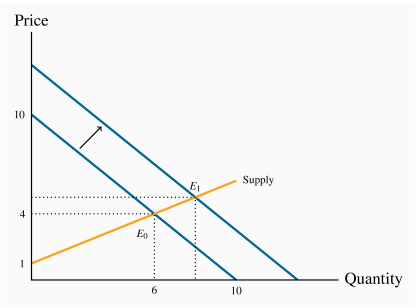
The demand curve in Figure 3.2 is drawn for a given level of other prices, incomes, tastes, and expectations. Movements along the demand curve reflect solely the impact of different prices for the good in question, holding other influences constant. But changes in any of these other factors will change the position of the demand curve. Figure 3.3 illustrates a shift in the demand curve. This shift could result from a rise in household incomes that increase the quantity demanded at every price. This is illustrated by an outward shift in the demand curve. With supply conditions unchanged, there is a new equilibrium at  , indicating a greater quantity of purchases accompanied by a higher price. The new equilibrium reflects a change in quantity supplied and a change in demand.
We may well ask why so much emphasis in our diagrams and analysis is placed on the relationship between price and quantity, rather than on the relationship between quantity and its other determinants. The answer is that we could indeed draw diagrams with quantity on the horizontal axis and a measure of one of these other influences on the vertical axis. But the price mechanism plays a very important role. Variations in price are what equilibrate the market. By focusing primarily upon the price, we see the self-correcting mechanism by which the market reacts to excess supply or excess demand.
In addition, this analysis illustrates the method of comparative statics—examining the impact of changing one of the other things that are assumed constant in the supply and demand diagrams.
Comparative static analysis compares an initial equilibrium with a new equilibrium, where the difference is due to a change in one of the other things that lie behind the demand curve or the supply curve.
'Comparative' obviously denotes the idea of a comparison, and static means that we are not in a state of motion. Hence we use these words in conjunction to indicate that we compare one outcome with another, without being concerned too much about the transition from an initial equilibrium to a new equilibrium. The transition would be concerned with dynamics rather than statics. In Figure 3.3 we explain the difference between the points E0 and E1 by indicating that there has been a change in incomes or in the price of a substitute good. We do not attempt to analyze the details of this move or the exact path from E0 to E1.
Application Box 3.1 Corn prices and demand shifts
In the middle of its second mandate, the Bush Administration in the US decided to encourage the production of ethanol – a fuel that is less polluting than gasoline. The target production was 35 billion for 2017 – from a base of 1 billion gallons in 2000. Corn is the principal input in ethanol production. It is also used as animal feed, as a sweetener and as a food for humans. The target was to be met with the help of a subsidy to producers and a tariff on imports of Brazil's sugar-cane based ethanol.
The impact on corn prices was immediate; from a farm-gate price of $2 per bushel in 2005, the price reached the $4 range two years later. In 2012 the price rose temporarily to $7. While other factors were in play - growing incomes and possibly speculation by commodity investors, ethanol is seen as the main price driver: demand for corn increased and the supply could not be increased to keep up with the demand without an increase in price.
The wider impact of these developments was that the prices of virtually all grains increased in tandem with corn: the prices of sorghum and barley increased because of a switch in land use towards corn on account of its profitability.
While farmers benefited from the price rise, consumers – particularly those in less developed economies – experienced a dramatic increase in their basic living costs. Visit the site of the United Nations' Food and Agricultural Organization for an assessment. Since hitting $7 per bushel in 2012, the price has dropped and averaged $3.50 in 2016.
In terms of supply and demand shifts: the demand side has dominated, particularly in the short run. The ethanol drive, combined with secular growth in the demand for food, means that the demand for grains shifted outward faster than the supply. In the period 2013–2016, supply has increased and the price has moderated.