To date we have drawn supply curves with an upward slope. Is this a reasonable representation of supply in view of what is frequently observed in markets? We suggested earlier that the various producers of a particular good or service may have different levels of efficiency. If so, only the more efficient producers can make a profit at a low price, whereas at higher prices more producers or suppliers enter the market – producers who may not be as lean and efficient as those who can survive in a lower-price environment. This view of the world yields a positively-sloping supply curve.
As a second example, consider Uber or Lyft taxi drivers. Some drivers may be in serious need of income and may be willing to drive for a low hourly rate. For other individuals driving may be a secondary source of income, and such drivers are less likely to want to drive unless the hourly wage is higher. Consequently if these ride sharing services need a large number of drivers at any one time it may be necessary to pay a higher wage – and charge a higher fare to passengers, to induce more drivers to take their taxis onto the road. This phenomenon corresponds to a positively-sloped supply curve.
In contrast to these two examples, some suppliers simply choose a unique price and let buyers purchase as much as they want at that price. This is the practice of most retailers. For example, the price of Samsung's Galaxy is typically fixed, no matter how many are purchased – and tens of millions are sold at a fixed price when a new model is launched. Apple also sets a price, and buyers purchase as many as they desire at that price. This practice corresponds to a horizontal supply curve: The price does not vary and the market equilibrium occurs where the demand curve intersects this supply curve.
In yet other situations supply is fixed. This happens in auctions. Bidders at the auction simply determine the price to be paid. At a real estate auction a given property is put on the market and the price is determined by the bidding process. In this case the supply of a single property is represented by a vertical supply at a quantity of 1 unit.
Regardless of the type of market we encounter, however, it is safe to assume that supply curves rarely slope downward. So, for the moment, we adopt the stance that supply curves are generally upward sloping – somewhere between the extremes of being vertical or horizontal – as we have drawn them to this point.
Next, we examine those other influences that underlie supply curves. Technology, input costs, the prices of competing goods, expectations and the number of suppliers are the most important.
Technology – computers and fracking
A technological advance may involve an idea that allows more output to be produced with the same inputs, or an equal output with fewer inputs. A good example is just-in-time technology. Before the modern era, virtually all manufacturers kept large stocks of components in their production facilities, but developments in communications and computers at that time made it possible for manufacturers to link directly with their input suppliers. Nowadays auto assembly plants place their order for, say, seat delivery to their local seat supplier well ahead of assembly time. The seats swing into the assembly area hours or minutes before assembly—just in time. The result is that the assembler reduces her seat inventory (an input) and thereby reduces production cost.
Such a technology-induced cost saving is represented by moving the supply curve downward or outward: The supplier is now able and willing to supply the same quantity at a lower price because of the technological innovation. Or, saying the same thing slightly differently, suppliers will supply more at a given price than before.
A second example relates to the extraction of natural gas. The development of 'fracking' means that companies involved in gas recovery can now do so at a lower cost. Hence they are willing to supply any given quantity at a lower price. A third example concerns aluminum cans. Today they weigh a fraction of what they weighed 20 years ago. This is a technology-based cost saving.
Input costs
Input costs can vary independently of technology. For example, a wage negotiation that grants workers a substantial pay raise will increase the cost of production. This is reflected in a leftward, or upward, supply shift: Any quantity supplied is now priced higher; alternatively, suppliers are willing to supply less at the going price.
Production costs may increase as a result of higher required standards in production. As governments implement new safety or product-stress standards, costs may increase. In this instance the increase in costs is not a 'bad' outcome for the buyer. She may be purchasing a higher quality good as a result.
Competing products – Airbnb versus hotels
If competing products improve in quality or fall in price, a supplier may be forced to follow suit. For example, Asus and Dell are constantly watching each other's pricing policies. If Dell brings out a new generation of computers at a lower price, Asus may lower its prices in turn—which is to say that Asus' supply curve will shift downward. Likewise, Samsung and Apple each responds to the other's pricing and technology behaviours. The arrival of new products in the marketplace also impacts the willingness of suppliers to supply goods at a given price. New intermediaries such as Airbnb and Vacation Rentals by Owner have shifted the supply curves of hotel rooms downward.
These are some of the many factors that influence the position of the supply curve in a given market.
Application Box 3.2 The price of light
Technological developments have had a staggering impact on many price declines. Professor William Nordhaus of Yale University is an expert on measuring technological change. He has examined the trend in the real price of lighting. Originally, light was provided by whale oil and gas lamps and these sources of lumens (the scientific measure of the amount of light produced) were costly. In his research, Professor Nordhaus pieced together evidence on the actual historic cost of light produced at various times, going all the way back to 1800. He found that light in 1800 cost about 100 times more than in 1900, and light in the year 2000 was a fraction of its cost in 1900. A rough calculation suggests that light was five hundred times more expensive at the start of this 200-year period than at the end, and this was before the arrival of LEDs.
In terms of supply and demand analysis, light has been subject to very substantial downward supply shifts. Despite the long-term growth in demand, the technologically-induced supply changes have been the dominant factor in its price determination.
For further information, visit Professor Nordhaus's website in the Department of Economics at Yale University.
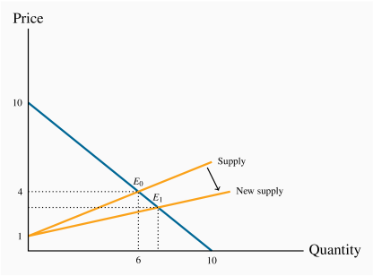
Shifts in supply
Whenever technology changes, or the costs of production change, or the prices of competing products adjust, then one of our ceteris paribus assumptions is violated. Such changes are generally reflected by shifting the supply curve. Figure 3.4 illustrates the impact of the arrival of just-in-time technology. The supply curve shifts, reflecting the ability of suppliers to supply the same output at a reduced price. The resulting new equilibrium price is lower, since production costs have fallen. At this reduced price more gas is traded at a lower price.