4: Measures of response- Elasticities

4.1 Price responsiveness of demand

Put yourself in the position of an entrepreneur. One of your many challenges is to price your product appropriately. You may be Michael Dell choosing a price for your latest computer, or the local restaurant owner pricing your table d'hôte, or you may be pricing your part-time snow-shoveling service. A key component of the pricing decision is to know how responsive your market is to variations in your pricing. How we measure responsiveness is the subject matter of this chapter.

We begin by analyzing the responsiveness of consumers to price changes. For example, consumers tend not to buy much more or much less food in response to changes in the general price level of food. This is because food is a pretty basic item for our existence. In contrast, if the price of new textbooks becomes higher, students may decide to search for a second-hand copy, or make do with lecture notes from their friends or downloads from the course web site. In the latter case students have ready alternatives to the new text book, and so their expenditure patterns can be expected to reflect these options, whereas it is hard to find alternatives to food. In the case of food consumers are not very responsive to price changes; in the case of textbooks they are. The word 'elasticity' that appears in this chapter title is just another term for this concept of responsiveness. Elasticity has many different uses and interpretations, and indeed more than one way of being measured in any given situation. Let us start by developing a suitable numerical measure.

The slope of the demand curve suggests itself as one measure of responsiveness: If we lowered the price of a good by $1, for example, how many more units would we sell? The difficulty with this measure is that it does not serve us well when comparing different products. One dollar may be a substantial part of the price of your morning coffee and croissant, but not very important if buying a computer or tablet. Accordingly, when goods and services are measured in different units (croissants versus tablets), or when their prices are very different, it is often best to use a percentage change measure, which is unit-free.

The price elasticity of demand is measured as the percentage change in quantity demanded, divided by the percentage change in price. Although we introduce several other elasticity measures later, when economists speak of the demand elasticity they invariably mean the price elasticity of demand defined in this way.

The price elasticity of demand can be written in different forms. We will use the Greek letter epsilon, , as a shorthand symbol, with a subscript d to denote demand, and the capital delta, , to denote a change. Therefore, we can write

or, using a shortened expression,

(4.1)

Calculating the value of the elasticity is not difficult. If we are told that a 10 percent price increase reduces the quantity demanded by 20 percent, then the elasticity value is The negative sign denotes that price and quantity move in opposite directions, but for brevity the negative sign is often omitted.

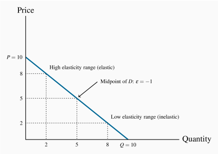
Consider now the data in Table 4.1 and the accompanying Figure 4.1. These data reflect the demand relation for natural gas that we introduced in Chapter 3. Note first that, when the price and quantity change, we must decide what reference price and quantity to use in the percentage change calculation in the definition above. We could use the initial or final price-quantity combination, or an average of the two. Each choice will yield a slightly different numerical value for the elasticity. The best convention is to use the midpoint of the price values and the corresponding midpoint of the quantity values. This ensures that the elasticity value is the same regardless of whether we start at the higher price or the lower price. Using the subscript 1 to denote the initial value and 2 the final value:

Figure 4.1 Elasticity variation with linear demand

In the high-price region of the demand curve the elasticity takes on a high value. At the midpoint of a linear demand curve the elasticity takes on a value of one, and at lower prices the elasticity value continues to fall.

Using this rule, consider now the value of when price drops from $10.00 to $8.00. The change in price is $2.00 and the average price is therefore . On the quantity side, demand goes from zero to 2 units (measured in thousands of cubic feet), and the average quantity demanded is therefore (0+2)/2=1. Putting these numbers into the formula yields:

Note that the price has declined in this instance and thus the change in price is negative. Continuing down the table in this fashion yields the full set of elasticity values in the third column.

The demand elasticity is said to be high if it is a large negative number; the large number denotes a high degree of sensitivity. Conversely, the elasticity is low if it is a small negative number. High and low refer to the size of the number, ignoring the negative sign. The term arc elasticity is also used to define what we have just measured, indicating that it defines consumer responsiveness over a segment or arc of the demand curve.

It is helpful to analyze this numerical example by means of the corresponding demand curve that is plotted in Figure 4.1, and which we used in Chapter 3. It is a straight-line demand curve; but, despite this, the elasticity is not constant. At high prices the elasticity is high; at low prices it is low. The intuition behind this pattern is as follows. When the price is high, a given price change represents a small percentage change, because the average price in the price-term denominator is large. At high prices the quantity demanded is small and therefore the percentage quantity change tends to be large due to the small quantity value in its denominator. In sum, at high prices the elasticity is large; it contains a large numerator and a small denominator. By the same reasoning, at low prices the elasticity is small.

We can carry this reasoning one step further to see what happens when the demand curve intersects the axes. At the horizontal axis the average price is tending towards zero. Since this extremely small value appears in the denominator of the price term it means that the price term as a whole is extremely large. Accordingly, with an extremely large value in the denominator of the elasticity expression, the whole ratio is tending towards a zero value. By the same reasoning the elasticity value at the vertical intercept is tending towards an infinitely large value.

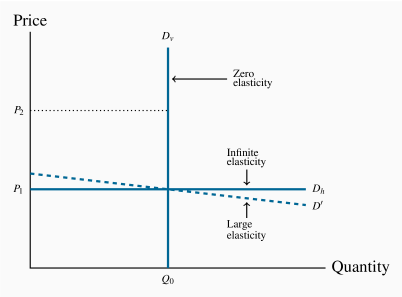
Extreme cases

The elasticity decreases in going from high prices to low prices. This is true for most non-linear demand curves also. Two exceptions are when the demand curve is horizontal and when it is vertical.

When the demand curve is vertical, no quantity change results from a change in price from P₁ to P₂, as illustrated in Figure 4.2 using the demand curve D_v. Therefore, the numerator in Equation 4.1 is zero, and the elasticity has a zero value.

Figure 4.2 Limiting cases of price elasticity

When the demand curve is vertical (D_v), the elasticity is zero: A change in price from P₁ to P₂ has no impact on the quantity demanded because the numerator in the elasticity formula has a zero value. When D becomes more horizontal the elasticity becomes larger and larger at P₁, eventually becoming infinite.

In the horizontal case, we say that the elasticity is infinite, which means that any percentage price change brings forth an infinite quantity change! This case is also illustrated in Figure 4.2 using the demand curve D_h. As with the vertical demand curve, this is not immediately obvious. So consider a demand curve that is almost horizontal, such as instead of D_h. In this instance, we can achieve large changes in quantity demanded by implementing very small price changes. In terms of Equation 4.1, the numerator is large and the denominator small, giving rise to a large elasticity. Now imagine that this demand curve becomes ever more elastic (horizontal). The same quantity response can be obtained with a smaller price change, and hence the elasticity is larger. Pursuing this idea, we can say that, as the demand curve becomes ever more elastic, the elasticity value tends towards infinity.

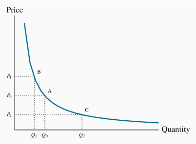
A non-linear demand curve is illustrated in Figure 4.3. If price increases from P₀ to P₁, the corresponding quantity change is given by (Q₀–Q₁). When the price declines to P₂ the quantity increases from Q₀ to Q₂. When statisticians study data to determine how responsive purchases are to price changes they do not always find a linear relationship between price and quantity. But a linear relationship is frequently a good approximation or representation of actual data and we will continue to analyze responsiveness in a linear framework in this chapter.

Figure 4.3 Non-linear demand curves

When the demand curve is non-linear the slope changes with the price. Hence, equal price changes do not lead to equal quantity changes: The quantity change associated with a change in price from P₀ to P₁ is smaller than the change in quantity associated with the same change in price from P₀ to P₂.

4.2 Price elasticities and public policy

In Chapter 3 we explored the implications of putting price floors and supply quotas in place. We saw that price floors can lead to excess supply. An important public policy question therefore is why these policies actually exist. It turns out that we can understand why with the help of elasticity concepts.

Price elasticity and expenditure

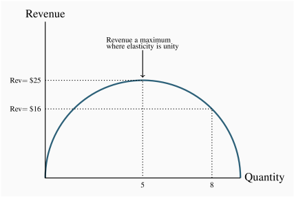
Let us return to Table 4.1 and explore what happens to total expenditure/revenue as the price varies. Since total revenue is simply the product of price times quantity it can be computed from the first two columns. The result is given in the final column. We see immediately that total expenditure on the good is highest at the midpoint of the demand curve corresponding to these data. At a price of $5 expenditure is $25. No other price yields more expenditure or revenue. Obviously the value $5 is midway between the zero value and the price or quantity intercept of the demand curve in Figure 4.1. This is a general result for linear demand curves: Expenditure is greatest at the midpoint, and the mid-price corresponds to the mid-quantity on the horizontal axis.

Geometrically this can be seen from Figure 4.1. Since expenditure is the product of price and quantity, in geometric terms it is the area of the rectangle mapped out by any price-quantity combination. For example, at total expenditure is $16 – the area of the rectangle bounded by these price and quantity values. Following this line of reasoning, if we were to compute the area bounded by a price of $7 and a corresponding quantity of 3 units we get a larger rectangle – a value of $21. This example indicates that the largest rectangle occurs at the midpoint of the demand curve. As a general geometric rule this is always the case. Hence we can conclude that the price that generates the greatest expenditure is the midpoint of a linear demand curve.

Let us now apply this rule to pricing in the market place. If our existing price is high and our goal is to generate more revenue, then we should reduce the price. Conversely, if our price is low and our goal is again to increase revenue we should raise the price. Starting from a high price let us see why this is so. By lowering the price we induce an increase in quantity demanded. Of course the lower price reduces the revenue obtained on the units already being sold at the initial high price. But since total expenditure increases at the new lower price, it must be the case that the additional sales caused by the lower price more than compensate for this loss on the units being sold at the initial high price. But there comes a point when this process ceases. Eventually the loss in revenue on the units being sold at the higher price is not offset by the revenue from additional quantity. We lose a margin on so many existing units that the additional sales cannot compensate. Accordingly revenue falls.

Note next that the top part of the demand curve is elastic and the lower part is inelastic. So, as a general rule we can state that:

A price decline (quantity increase) on an elastic segment of a demand curve necessarily increases revenue, and a price increase (quantity decline) on an inelastic segment also increases revenue.

The result is mapped in Figure 4.4, which plots total revenue as a function of the quantity demanded – columns 2 and 4 from Table 4.1. At low quantity values the price is high and the demand is elastic; at high quantity values the price is low and the demand is inelastic. The revenue maximizing point is the midpoint of the demand curve.

Figure 4.4 Total revenue and elasticity

Based upon the data in Table 4.1, revenue increases with quantity sold up to sales of 5 units. Beyond this output, the decline in price that must accompany additional sales causes revenue to decline.

We now have a general conclusion: In order to maximize the possible revenue from the sale of a good or service, it should be priced where the demand elasticity is unity.

Does this conclusion mean that every entrepreneur tries to find this magic region of the demand curve in pricing her product? Not necessarily: Most businesses seek to maximize their profit rather than their revenue, and so they have to focus on cost in addition to sales. We will examine this interaction in later chapters. Secondly, not every firm has control over the price they charge; the price corresponding to the unit elasticity may be too high relative to their competitors' price choices. Nonetheless, many firms, especially in the early phase of their life-cycle, focus on revenue growth rather than profit, and so, if they have any power over their price, the choice of the unit-elastic price may be appropriate.

The agriculture problem

We are now in a position to address the question we posed above: Why are price floors frequently found in agricultural markets? The answer is that governments believe that the pressures of competition would force farm/food prices so low that many farmers would not be able to earn a reasonable income from farming. Accordingly, governments impose price floors. Keep in mind that price floors are prices above the market equilibrium and therefore lead to excess supply.

Since the demand for foodstuffs is inelastic we know that a higher price will induce more revenue, even with a lower quantity being sold. The government can force this outcome on the market by a policy of supply management. It can force farmers in the aggregate to bring only a specific amount of product to the market, and thus ensure that the price floor does not lead to excess supply. This is the system of supply management we observe in dairy markets in Canada, for example, and that we examined in the case of maple syrup in Chapter 3. Its supporters praise it because it helps farmers, its critics point out that higher food prices hurt lower-income households more than high-income households, and therefore it is not a good policy.

Elasticity values are frequently more informative than diagrams and figures. Our natural inclination is to view demand curves with a somewhat vertical profile as being inelastic, and demand curves with a flatter profile as elastic. But we must keep in mind that, as explained in Chapter 2, the vertical and horizontal axis of any diagram can be scaled in such a way as to change the visual impact of the data underlying the curves. But a numerical elasticity value will never deceive in this way. If its value is less than unity it is inelastic, regardless of the visual aspect of the demand curve.

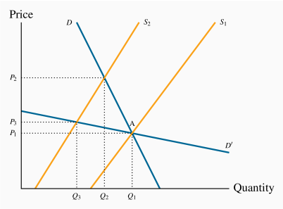
At the same time, if we have two demand curves intersecting at a particular price-quantity combination, we can say that the curve with the more vertical profile is relatively more elastic, or less inelastic. This is illustrated in Figure 4.5. It is clear that, at the price-quantity combination where they intersect, the demand curve will yield a greater (percentage) quantity change than the demand curve D, for a given (percentage) price change. Hence, on the basis of diagrams, we can compare demand elasticities in relative terms at a point where the two intersect.

Figure 4.5 The impact of elasticity on quantity fluctuations

In the lower part of the demand curve D, demand is inelastic: At the point A, a shift in supply from S₁ to S₂ induces a large percentage increase in price, and a small percentage decrease in quantity demanded. In contrast, for the demand curve that goes through the original equilibrium, the region A is now an elastic region, and the impact of the supply shift is contrary: The % is smaller and the % is larger.

4.3 The time horizon and inflation

The price elasticity of demand is frequently lower in the short run than in the long run. For example, a rise in the price of home heating oil may ultimately induce consumers to switch to natural gas or electricity, but such a transition may require a considerable amount of time. Time is required for decision-making and investment in new heating equipment. A further example is the elasticity of demand for tobacco. Some adults who smoke may be seriously dependent and find quitting almost impossible. Higher prices may provide a stronger incentive to reduce or quit, but successful quitters usually require several attempts before being successful. Several years may be required for the impact of a price increase to be fully apparent. Accordingly when we talk of the short run and the long run, there is no simple rule for defining how long the long run actually is in terms of months or years. In some cases, adjustment may be complete in weeks, in other cases years.

In Chapter 2 we distinguished between real and nominal variables. The former adjust for inflation; the latter do not. Suppose all nominal variables double in value: Every good and service costs twice as much, wage rates double, dividends and rent double, etc. This implies that whatever bundle of goods was previously affordable is still affordable. Nothing has really changed. Demand behaviour is unaltered by this doubling of all prices and all incomes.

How do we reconcile this with the idea that own-price elasticities measure changes in quantity demanded as prices change? Keep in mind that elasticities measure the impact of changing one variable alone, holding constant all of the others. But when all variables are changing simultaneously, it is incorrect to think that the impact on quantity of one price or income change is a true measure of responsiveness or elasticity. The price changes that go into measuring elasticities are therefore changes in prices relative to inflation.

4.4 Cross-price elasticities – cable or satellite

The price elasticity of demand tells us about consumer responses to price changes in different regions of the demand curve, holding constant all other influences. One of those influences is the price of other goods and services. A cross-price elasticity indicates how demand is influenced by changes in the prices of other products.

We write the cross price elasticity of the demand for x due to a change in the price of y as

For example, if the price of cable-supply internet services declines, by how much will the demand for satellite-supply services change? The cross-price elasticity may be positive or negative. These particular goods are clearly substitutable, and this is reflected in a positive value of this cross-price elasticity: The percentage change in satellite subscribers will be negative in response to a decline in the price of cable; a negative divided by a negative is positive. In contrast, a change in the price of tablets or electronic readers should induce an opposing change in the quantity of e-books purchased: Lower tablet prices will induce greater e-book purchases. In this case the price and quantity movements are in opposite directions and the elasticity is therefore negative – the goods are complements.

4.5 The income elasticity of demand

In Chapter 3 we stated that higher incomes tend to increase the quantity demanded at any price. To measure the responsiveness of demand to income changes, a unit-free measure exists: The income elasticity of demand. The income elasticity of demand is the percentage change in quantity demanded divided by a percentage change in income.

Let us use the Greek letter eta, , to define the income elasticity of demand and I to denote income. Then,

As an example, if monthly income increases by 10 percent, and the quantity of magazines purchased increases by 15 percent, then the income elasticity of demand for magazines is 1.5 in value . The income elasticity is generally positive, but not always – let us see why.

Normal, inferior, necessary, and luxury goods

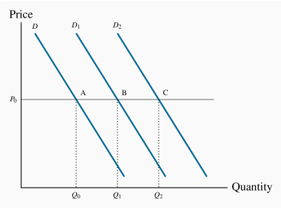
The income elasticity of demand, in diagrammatic terms, is a percentage measure of how far the demand curve shifts in response to a change in income. Figure 4.6 shows two possible shifts. Suppose the demand curve is initially the one defined by D, and then income increases. In this example the supply curve is horizontal at the price P₀. If the demand curve shifts to D₁ as a result, the change in quantity demanded at the existing price is (Q₁–Q₀). However, if instead the demand curve shifts to D₂, that shift denotes a larger change in quantity (Q₂–Q₀). Since the shift in demand denoted by D₂ exceeds the shift to D₁, the D₂ shift is more responsive to income, and therefore implies a higher income elasticity.

Figure 4.6 Income elasticity and shifts in demand

At the price P₀, the income elasticity measures the percentage horizontal shift in demand caused by some percentage income increase. A shift from A to B reflects a lower income elasticity than a shift to C. A leftward shift in the demand curve in response to an income increase would denote a negative income elasticity – an inferior good.

In this example, the good is a normal good, as defined in Chapter 3, because the demand for it increases in response to income increases. If the demand curve were to shift back to the left in response to an increase in income, then the income elasticity would be negative. In such cases the goods or services are inferior, as defined in Chapter 3.

Finally, we distinguish between luxuries and necessities. A luxury good or service is one whose income elasticity equals or exceeds unity. A necessity is one whose income elasticity is greater than zero but less than unity. If quantity demanded is so responsive to an income increase that the percentage increase in quantity demanded exceeds the percentage increase in income, then the elasticity value is in excess of 1, and the good or service is called a luxury. In contrast, if the percentage change in quantity demanded is less than the percentage increase in income, the value is less than unity, and we call the good or service a necessity.

A luxury good or service is one whose income elasticity equals or exceeds unity.

A necessity is one whose income elasticity is greater than zero and less than unity.

Luxuries and necessities can also be defined in terms of their share of a typical budget. An income elasticity greater than unity means that the share of an individual's budget being allocated to the product is increasing. In contrast, if the elasticity is less than unity, the budget share is falling. This makes intuitive sense—luxury cars are luxury goods by this definition because they take up a larger share of the incomes of the rich than the non-rich.

Inferior goods are those for which there exist higher-quality, more expensive, substitutes. For example, lower-income households tend to satisfy their travel needs by using public transit. As income rises, households may reduce their reliance on public transit in favour of automobile use (despite the congestion and environmental impacts). Likewise, laundromats are inferior goods in the sense that, as income increases, individuals tend to purchase their own appliances and therefore use laundromat services less. Inferior goods, therefore, have a negative income elasticity: In the income elasticity equation definition, the numerator has a sign opposite to that of the denominator.

Inferior goods have negative income elasticity.

Empirical research indicates that goods like food and fuel have income elasticities less than 1; durable goods and services have elasticities slightly greater than 1; leisure goods and foreign holidays have elasticities very much greater than 1.

Income elasticities are useful in forecasting the demand for particular services and goods in a growing economy. Suppose real income is forecast to grow by 15% over the next five years. If we know that the income elasticity of demand for smart phones is 2.0, we could estimate the anticipated growth in demand by using the income elasticity formula: Since in this case and it follows that . Therefore the predicted demand change must be 30%.

4.6 Elasticity of supply

Now that we have developed the various dimensions of elasticity on the demand side, the analysis of elasticities on the supply side is straightforward. The elasticity of supply measures the responsiveness of the quantity supplied to a change in the price.

The subscript s denotes supply. This is exactly the same formula as for the demand curve, except that the quantities now come from a supply curve. Furthermore, and in contrast to the demand elasticity, the supply elasticity is generally a positive value because of the positive relationship between price and quantity supplied. The more elastic, or the more responsive, is supply to a given price change, the larger will be the elasticity value. In diagrammatic terms, this means that "flatter" supply curves have a greater elasticity than more "vertical" curves at a given price and quantity combination. Numerically the flatter curve has a larger value than the more vertical supply – try drawing a supply diagram similar to Figure 4.2. Technically, a completely vertical supply curve has a zero elasticity and a horizontal supply curve has an infinite elasticity – just as in the demand cases.

As always we keep in mind the danger of interpreting too much about the value of this elasticity from looking at the visual profiles of supply curves.

Application Box 4.2 The price of oil and the coronavirus

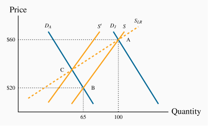
In January 2020, the price of oil in the US traded at $60 per barrel. The coronavirus then struck the world economy, transport declined dramatically, and by the beginning of April the price had dropped to $20 per barrel. The quantity of oil traded on world markets fell from approximately 100 million barrels per day in January to 65 million barrels by the start of April, a drop of 35% relative to its January level. This scenario is displayed in Figure 4.7 below.

Figure 4.7 Supply elasticity in the short run and the long run; the oil market in 2020

Demand drops suddenly between January and April. Equilibrium moves from point A to B. In the long run some producers exit and the supply curve shifts towards the origin. Following this, the equilibrium is C. Joining points such as A and C yields a long run supply curve; it is more elastic than the short run supply, when the number of suppliers is fixed.

The January equilibrium is at the point A, and the April equilibrium at point B. The move from A to B was caused by a collapse in demand as illustrated by the shift in the demand curve. We can compute the supply elasticity readily from this example. Note that it was demand that shifted rather than supply so we are observing two points on the supply curve. The supply elasticity, using arc values, is given by (35/82.5)/($40/$40) = 0.42. So the supply curve is inelastic.

Can all oil producers survive in this bear market? The answer is no. It is inexpensive to pump oil in Saudi Arabia, but more costly to produce it from shale or tar sands, and thus some producers are not covering their costs with the price at $20 per barrel. They do not want to shut their operations because closing down and reopening is expensive. They hang on in the hope that the price will return towards $60. If demand does not recover, some suppliers exit the industry with the passage of time. With fewer suppliers the supply curve shifts towards the origin and ultimately another equilibrium price and quantity are established. Call this new equilibrium point C.

The supply elasticity takes on a different value in the short run than in the long run. Supply is more inelastic in the short run. A line through the points A and C would represent the long-run supply curve for the industry. It must be more elastic than the short run supply because the industry has had time to adjust - it is more flexible with the passage of time.

4.7 Elasticities and tax incidence

Elasticity values are critical in determining the impact of a government's taxation policies. The spending and taxing activities of the government influence the use of the economy's resources. By taxing cigarettes, alcohol and fuel, the government can restrict their use; by taxing income, the government influences the amount of time people choose to work. Taxes have a major impact on almost every sector of the Canadian economy.

To illustrate the role played by demand and supply elasticities in tax analysis, we take the example of a sales tax. These can be of the specific or ad valorem type. A specific tax involves a fixed dollar levy per unit of a good sold (e.g., $10 per airport departure). An ad valorem tax is a percentage levy, such as Canada's Goods and Services tax (e.g., 5 percent on top of the retail price of goods and services). The impact of each type of tax is similar, and we will use the specific tax in our example below.

A layperson's view of a sales tax is that the tax is borne by the consumer. That is to say, if no sales tax were imposed on the good or service in question, the price paid by the consumer would be the same net of tax price as exists when the tax is in place. Interestingly, this is not always the case. The study of the incidence of taxes is the study of who really bears the tax burden, and this in turn depends upon supply and demand elasticities.

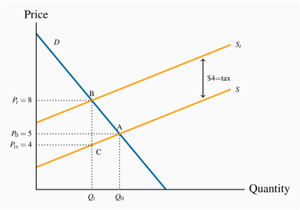
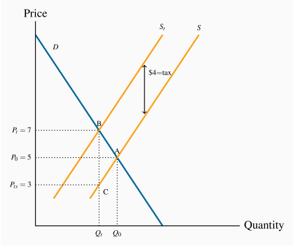
Consider Figures 4.8 and 4.9, which define an imaginary market for inexpensive wine. Let us suppose that, without a tax, the equilibrium price of a bottle of wine is $5, and Q₀ is the equilibrium quantity traded. The pre-tax equilibrium is at the point A. The government now imposes a specific tax of $4 per bottle. The impact of the tax is represented by an upward shift in supply of $4: Regardless of the price that the consumer pays, $4 of that price must be remitted to the government. As a consequence, the price paid to the supplier must be $4 less than the consumer price, and this is represented by twin supply curves: One defines the price at which the supplier is willing to supply (S), and the other is the tax-inclusive supply curve that the consumer faces (S_t).

Figure 4.8 Tax incidence with elastic supply

The imposition of a specific tax of $4 shifts the supply curve vertically by $4. The final price at B (P_t) increases by $3 over the equilibrium price at A. At the new quantity traded, Q_t, the supplier gets $4 per unit (), the government gets $4 also and the consumer pays $8. The greater part of the incidence is upon the buyer, on account of the relatively elastic supply curve: His price increases by $3 of the $4 tax.

The introduction of the tax in Figure 4.8 means that consumers now face the supply curve S_t. The new equilibrium is at point B. Note that the price has increased by less than the full amount of the tax—in this example it has increased by $3. This is because the reduced quantity at B is provided at a lower supply price: The supplier is willing to supply the quantity Q_t at a price defined by C ($4), which is lower than the price at A ($5).

So what is the incidence of the $4 tax? Since the market price has increased from $5 to $8, and the price obtained by the supplier has fallen by $1, we say that the incidence of the tax falls mainly on the consumer: The price to the consumer has risen by three dollars and the price received by the supplier has fallen by just one dollar.

Consider now Figure 4.9, where the supply curve is less elastic, and the demand curve is unchanged. Again the supply curve must shift upward with the imposition of the specific tax. But here the price received by the supplier is lower than in Figure 4.8, and the price paid by the consumer does not rise as much – the incidence is different. The consumer faces a price increase that is one-half, rather than three-quarters, of the tax value. The supplier faces a lower supply price, and bears a higher share of the tax.

Figure 4.9 Tax incidence with inelastic supply

The imposition of a specific tax of $4 shifts the supply curve vertically by $4. The final price at B (P_t) increases by $2 over the no-tax price at A. At the new quantity traded, Q_t, the supplier gets $3 per unit (), the government gets $4 also and the consumer pays $7. The incidence is shared equally by suppliers and demanders.

We can conclude from this example that, for any given demand, the more elastic is supply, the greater is the price increase in response to a given tax. Furthermore, a more elastic supply curve means that the incidence falls more on the consumer; while a less elastic supply curve means the incidence falls more on the supplier. This conclusion can be verified by drawing a third version of Figure 4.8 and 4.9, in which the supply curve is horizontal – perfectly elastic. When the tax is imposed the price to the consumer increases by the full value of the tax, and the full incidence falls on the buyer. While this case corresponds to the layperson's intuition of the incidence of a tax, economists recognize it as a special case of the more general outcome, where the incidence falls on both the supply side and the demand side.

These are key results in the theory of taxation. It is equally the case that the incidence of the tax depends upon the demand elasticity. In Figure 4.8 and 4.9 we used the same demand curve. However, it is not difficult to see that, if we were to redo the exercise with a demand curve of a different elasticity, the incidence would not be identical. At the same time, the general result on supply elasticities still holds. We will return to this material in Chapter 5.

4.8 Technical tricks with elasticities

We can easily compute elasticities at any point on a demand curve, rather than over a range or arc, by using the explicit formula for the demand curve. To see this note that we can rewrite Equation 4.1 as:

The first term in the final form of this expression is obtained from the slope of the demand curve, and the second term (P/Q) is defined by the point on the curve that interests us. For example if our demand curve is , then . Inverting this to get yields –1 also. So, the point elasticity value at is . This formula provides the elasticity value at a particular point on the demand curve, rather than over a range of values or an arc. Consequently it is called the point elasticity of demand. And obviously we could apply it to a demand curve that is not linear provided we know the mathematical form and are able to establish the slope.

Key Terms

Exercises for Chapter 4