Put yourself in the position of an entrepreneur. One of your many challenges is to price your product appropriately. You may be Michael Dell choosing a price for your latest computer, or the local restaurant owner pricing your table d'hôte, or you may be pricing your part-time snow-shoveling service. A key component of the pricing decision is to know how responsive your market is to variations in your pricing. How we measure responsiveness is the subject matter of this chapter.
We begin by analyzing the responsiveness of consumers to price changes. For example, consumers tend not to buy much more or much less food in response to changes in the general price level of food. This is because food is a pretty basic item for our existence. In contrast, if the price of new textbooks becomes higher, students may decide to search for a second-hand copy, or make do with lecture notes from their friends or downloads from the course web site. In the latter case students have ready alternatives to the new text book, and so their expenditure patterns can be expected to reflect these options, whereas it is hard to find alternatives to food. In the case of food consumers are not very responsive to price changes; in the case of textbooks they are. The word 'elasticity' that appears in this chapter title is just another term for this concept of responsiveness. Elasticity has many different uses and interpretations, and indeed more than one way of being measured in any given situation. Let us start by developing a suitable numerical measure.
The slope of the demand curve suggests itself as one measure of responsiveness: If we lowered the price of a good by $1, for example, how many more units would we sell? The difficulty with this measure is that it does not serve us well when comparing different products. One dollar may be a substantial part of the price of your morning coffee and croissant, but not very important if buying a computer or tablet. Accordingly, when goods and services are measured in different units (croissants versus tablets), or when their prices are very different, it is often best to use a percentage change measure, which is unit-free.
The price elasticity of demand is measured as the percentage change in quantity demanded, divided by the percentage change in price. Although we introduce several other elasticity measures later, when economists speak of the demand elasticity they invariably mean the price elasticity of demand defined in this way.
The price elasticity of demand is measured as the percentage change in quantity demanded, divided by the percentage change in price.
The price elasticity of demand can be written in different forms. We will use the Greek letter epsilon,  , as a shorthand symbol, with a subscript d to denote demand, and the capital delta,
  , to denote a change. Therefore, we can write
or, using a shortened expression,
 |
(4.1) |
Calculating the value of the elasticity is not difficult. If we are told that a 10 percent price increase reduces the quantity demanded by 20 percent, then the elasticity value is  The negative sign denotes that price and quantity move in opposite directions, but for brevity the negative sign is often omitted.
Consider now the data in Table 4.1 and the accompanying Figure 4.1. These data reflect the demand relation for natural gas that we introduced in Chapter 3. Note first that, when the price and quantity change, we must decide what reference price and quantity to use in the percentage change calculation in the definition above. We could use the initial or final price-quantity combination, or an average of the two. Each choice will yield a slightly different numerical value for the elasticity. The best convention is to use the midpoint of the price values and the corresponding midpoint of the quantity values. This ensures that the elasticity value is the same regardless of whether we start at the higher price or the lower price. Using the subscript 1 to denote the initial value and 2 the final value:


Table 4.1 The demand for natural gas: Elasticities and revenue
| Price ($) |
Quantity |
Elasticity |
Total |
| |
demanded |
value |
revenue ($) |
| 10 |
0 |
|
0 |
| 9 |
1 |
-9.0 |
9 |
| 8 |
2 |
|
16 |
| 7 |
3 |
-2.33 |
21 |
| 6 |
4 |
|
24 |
| 5 |
5 |
-1.0 |
25 |
| 4 |
6 |
|
24 |
| 3 |
7 |
-0.43 |
21 |
| 2 |
8 |
|
16 |
| 1 |
9 |
-0.11 |
9 |
| 0 |
10 |
|
0 |
Elasticity calculations are based upon $2 price changes.
Using this rule, consider now the value of  when price drops from $10.00 to $8.00. The change in price is $2.00 and the average price is therefore
 . On the quantity side, demand goes from zero to 2 units (measured in thousands of cubic feet), and the average quantity demanded is therefore (0+2)/2=1. Putting these numbers into the formula yields:
Note that the price has declined in this instance and thus the change in price is negative. Continuing down the table in this fashion yields the full set of elasticity values in the third column.
The demand elasticity is said to be high if it is a large negative number; the large number denotes a high degree of sensitivity. Conversely, the elasticity is low if it is a small negative number. High and low refer to the size of the number, ignoring the negative sign. The term arc elasticity is also used to define what we have just measured, indicating that it defines consumer responsiveness over a segment or arc of the demand curve.
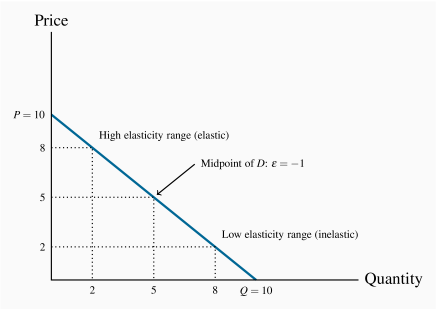
It is helpful to analyze this numerical example by means of the corresponding demand curve that is plotted in Figure 4.1, and which we used in Chapter 3. It is a straight-line demand curve; but, despite this, the elasticity is not constant. At high prices the elasticity is high; at low prices it is low. The intuition behind this pattern is as follows. When the price is high, a given price change represents a small percentage change, because the average price in the price-term denominator is large. At high prices the quantity demanded is small and therefore the percentage quantity change tends to be large due to the small quantity value in its denominator. In sum, at high prices the elasticity is large; it contains a large numerator and a small denominator. By the same reasoning, at low prices the elasticity is small.
We can carry this reasoning one step further to see what happens when the demand curve intersects the axes. At the horizontal axis the average price is tending towards zero. Since this extremely small value appears in the denominator of the price term it means that the price term as a whole is extremely large. Accordingly, with an extremely large value in the denominator of the elasticity expression, the whole ratio is tending towards a zero value. By the same reasoning the elasticity value at the vertical intercept is tending towards an infinitely large value.
Extreme cases
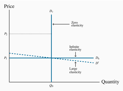
The elasticity decreases in going from high prices to low prices. This is true for most non-linear demand curves also. Two exceptions are when the demand curve is horizontal and when it is vertical.
When the demand curve is vertical, no quantity change results from a change in price from P1 to P2, as illustrated in Figure 4.2 using the demand curve Dv. Therefore, the numerator in Equation 4.1 is zero, and the elasticity has a zero value.
In the horizontal case, we say that the elasticity is infinite, which means that any percentage price change brings forth an infinite quantity change! This case is also illustrated in Figure 4.2 using the demand curve Dh. As with the vertical demand curve, this is not immediately obvious. So consider a demand curve that is almost horizontal, such as  instead of Dh. In this instance, we can achieve large changes in quantity demanded by implementing very small price changes. In terms of Equation 4.1, the numerator is large and the denominator small, giving rise to a large elasticity. Now imagine that this demand curve becomes ever more elastic (horizontal). The same quantity response can be obtained with a smaller price change, and hence the elasticity is larger. Pursuing this idea, we can say that, as the demand curve becomes ever more elastic, the elasticity value tends towards infinity.
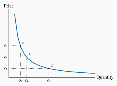
A non-linear demand curve is illustrated in Figure 4.3. If price increases from P0 to P1, the corresponding quantity change is given by (Q0–Q1). When the price declines to P2 the quantity increases from Q0 to Q2. When statisticians study data to determine how responsive purchases are to price changes they do not always find a linear relationship between price and quantity. But a linear relationship is frequently a good approximation or representation of actual data and we will continue to analyze responsiveness in a linear framework in this chapter.
Elastic and inelastic demands
While the elasticity value falls as we move down the demand curve, an important dividing line occurs at the value of –1. This is illustrated in Table 4.1, and is a property of all straight-line demand curves. Disregarding the negative sign, demand is said to be elastic if the price elasticity is greater than unity, and inelastic if the value lies between unity and 0. It is unit elastic if the value is exactly one.
Demand is elastic if the price elasticity is greater than unity. It is inelastic if the value lies between unity and 0. It is unit elastic if the value is exactly one.
Economists frequently talk of goods as having a "high" or "low" demand elasticity. What does this mean, given that the elasticity varies throughout the length of a demand curve? It signifies that, at the price usually charged, the elasticity has a high or low value. For example, your weekly demand for regular coffee at Starbucks might be unresponsive to variations in price around the value of $3.00, but if the price were $6, you might be more responsive to price variations. Likewise, when we stated at the beginning of this chapter that the demand for food tends to be inelastic, we really meant that at the price we customarily face for food, demand is inelastic.
Determinants of price elasticity
Why is it that the price elasticities for some goods and services are high and for others low?
- One answer lies in tastes: If a good or service is a basic necessity in one's life, then price variations have a minimal effect on the quantity demanded, and these products thus have a relatively inelastic demand.
- A second answer lies in the ease with which we can substitute alternative goods or services for the product in question. If Apple Corporation had no serious competition in the smart-phone market, it could price its products even higher than in the presence of Samsung and Google, who also supply smart phones. A supplier who increases her price will lose more sales if there are ready substitutes to which buyers can switch, than if no such substitutes exist. It follows that a critical role for the marketing department in a firm is to convince buyers of the uniqueness of the firm's product.
- Where product groups are concerned, the price elasticity of demand for one product is necessarily higher than for the group as a whole: Suppose the price of one computer tablet brand alone falls. Buyers would be expected to substitute towards this product in large numbers – its manufacturer would find demand to be highly responsive. But if all brands are reduced in price, the increase in demand for any one will be more muted. In essence, the one tablet whose price falls has several close substitutes, but tablets in the aggregate do not.
- Finally, there is a time dimension to responsiveness, and this is explored in Section 4.3.