4.5: The income elasticity of demand

In Chapter 3 we stated that higher incomes tend to increase the quantity demanded at any price. To measure the responsiveness of demand to income changes, a unit-free measure exists: The income elasticity of demand. The income elasticity of demand is the percentage change in quantity demanded divided by a percentage change in income.

The income elasticity of demand is the percentage change in quantity demanded divided by a percentage change in income.

Let us use the Greek letter eta, , to define the income elasticity of demand and I to denote income. Then,

As an example, if monthly income increases by 10 percent, and the quantity of magazines purchased increases by 15 percent, then the income elasticity of demand for magazines is 1.5 in value . The income elasticity is generally positive, but not always – let us see why.

Normal, inferior, necessary, and luxury goods

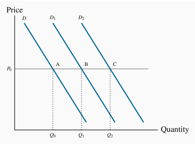
The income elasticity of demand, in diagrammatic terms, is a percentage measure of how far the demand curve shifts in response to a change in income. Figure 4.6 shows two possible shifts. Suppose the demand curve is initially the one defined by D, and then income increases. In this example the supply curve is horizontal at the price P₀. If the demand curve shifts to D₁ as a result, the change in quantity demanded at the existing price is (Q₁–Q₀). However, if instead the demand curve shifts to D₂, that shift denotes a larger change in quantity (Q₂–Q₀). Since the shift in demand denoted by D₂ exceeds the shift to D₁, the D₂ shift is more responsive to income, and therefore implies a higher income elasticity.

Figure 4.6 Income elasticity and shifts in demand

At the price P₀, the income elasticity measures the percentage horizontal shift in demand caused by some percentage income increase. A shift from A to B reflects a lower income elasticity than a shift to C. A leftward shift in the demand curve in response to an income increase would denote a negative income elasticity – an inferior good.

In this example, the good is a normal good, as defined in Chapter 3, because the demand for it increases in response to income increases. If the demand curve were to shift back to the left in response to an increase in income, then the income elasticity would be negative. In such cases the goods or services are inferior, as defined in Chapter 3.

Finally, we distinguish between luxuries and necessities. A luxury good or service is one whose income elasticity equals or exceeds unity. A necessity is one whose income elasticity is greater than zero but less than unity. If quantity demanded is so responsive to an income increase that the percentage increase in quantity demanded exceeds the percentage increase in income, then the elasticity value is in excess of 1, and the good or service is called a luxury. In contrast, if the percentage change in quantity demanded is less than the percentage increase in income, the value is less than unity, and we call the good or service a necessity.

A luxury good or service is one whose income elasticity equals or exceeds unity.

A necessity is one whose income elasticity is greater than zero and less than unity.

Luxuries and necessities can also be defined in terms of their share of a typical budget. An income elasticity greater than unity means that the share of an individual's budget being allocated to the product is increasing. In contrast, if the elasticity is less than unity, the budget share is falling. This makes intuitive sense—luxury cars are luxury goods by this definition because they take up a larger share of the incomes of the rich than the non-rich.

Inferior goods are those for which there exist higher-quality, more expensive, substitutes. For example, lower-income households tend to satisfy their travel needs by using public transit. As income rises, households may reduce their reliance on public transit in favour of automobile use (despite the congestion and environmental impacts). Likewise, laundromats are inferior goods in the sense that, as income increases, individuals tend to purchase their own appliances and therefore use laundromat services less. Inferior goods, therefore, have a negative income elasticity: In the income elasticity equation definition, the numerator has a sign opposite to that of the denominator.

Inferior goods have negative income elasticity.

Empirical research indicates that goods like food and fuel have income elasticities less than 1; durable goods and services have elasticities slightly greater than 1; leisure goods and foreign holidays have elasticities very much greater than 1.

Income elasticities are useful in forecasting the demand for particular services and goods in a growing economy. Suppose real income is forecast to grow by 15% over the next five years. If we know that the income elasticity of demand for smart phones is 2.0, we could estimate the anticipated growth in demand by using the income elasticity formula: Since in this case and it follows that . Therefore the predicted demand change must be 30%.