4.6: Elasticity of supply

Last updated
Save as PDF

Page ID: 108380

$ \newcommand{\vecs}[1]{\overset { \scriptstyle \rightharpoonup} {\mathbf{#1}} } $ $ \newcommand{\vecd}[1]{\overset{-\!-\!\rightharpoonup}{\vphantom{a}\smash {#1}}} $$\newcommand{\id}{\mathrm{id}}$ $ \newcommand{\Span}{\mathrm{span}}$ $ \newcommand{\kernel}{\mathrm{null}\,}$ $ \newcommand{\range}{\mathrm{range}\,}$ $ \newcommand{\RealPart}{\mathrm{Re}}$ $ \newcommand{\ImaginaryPart}{\mathrm{Im}}$ $ \newcommand{\Argument}{\mathrm{Arg}}$ $ \newcommand{\norm}[1]{\| #1 \|}$ $ \newcommand{\inner}[2]{\langle #1, #2 \rangle}$ $ \newcommand{\Span}{\mathrm{span}}$ $\newcommand{\id}{\mathrm{id}}$ $ \newcommand{\Span}{\mathrm{span}}$ $ \newcommand{\kernel}{\mathrm{null}\,}$ $ \newcommand{\range}{\mathrm{range}\,}$ $ \newcommand{\RealPart}{\mathrm{Re}}$ $ \newcommand{\ImaginaryPart}{\mathrm{Im}}$ $ \newcommand{\Argument}{\mathrm{Arg}}$ $ \newcommand{\norm}[1]{\| #1 \|}$ $ \newcommand{\inner}[2]{\langle #1, #2 \rangle}$ $ \newcommand{\Span}{\mathrm{span}}$$\newcommand{\AA}{\unicode[.8,0]{x212B}}$

Now that we have developed the various dimensions of elasticity on the demand side, the analysis of elasticities on the supply side is straightforward. The elasticity of supply measures the responsiveness of the quantity supplied to a change in the price.

The elasticity of supply measures the responsiveness of quantity supplied to a change in the price.

The subscript s denotes supply. This is exactly the same formula as for the demand curve, except that the quantities now come from a supply curve. Furthermore, and in contrast to the demand elasticity, the supply elasticity is generally a positive value because of the positive relationship between price and quantity supplied. The more elastic, or the more responsive, is supply to a given price change, the larger will be the elasticity value. In diagrammatic terms, this means that "flatter" supply curves have a greater elasticity than more "vertical" curves at a given price and quantity combination. Numerically the flatter curve has a larger value than the more vertical supply – try drawing a supply diagram similar to Figure 4.2. Technically, a completely vertical supply curve has a zero elasticity and a horizontal supply curve has an infinite elasticity – just as in the demand cases.

As always we keep in mind the danger of interpreting too much about the value of this elasticity from looking at the visual profiles of supply curves.

Application Box 4.2 The price of oil and the coronavirus

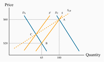
In January 2020, the price of oil in the US traded at $60 per barrel. The coronavirus then struck the world economy, transport declined dramatically, and by the beginning of April the price had dropped to $20 per barrel. The quantity of oil traded on world markets fell from approximately 100 million barrels per day in January to 65 million barrels by the start of April, a drop of 35% relative to its January level. This scenario is displayed in Figure 4.7 below.

Figure 4.7 Supply elasticity in the short run and the long run; the oil market in 2020

Demand drops suddenly between January and April. Equilibrium moves from point A to B. In the long run some producers exit and the supply curve shifts towards the origin. Following this, the equilibrium is C. Joining points such as A and C yields a long run supply curve; it is more elastic than the short run supply, when the number of suppliers is fixed.

The January equilibrium is at the point A, and the April equilibrium at point B. The move from A to B was caused by a collapse in demand as illustrated by the shift in the demand curve. We can compute the supply elasticity readily from this example. Note that it was demand that shifted rather than supply so we are observing two points on the supply curve. The supply elasticity, using arc values, is given by (35/82.5)/($40/$40) = 0.42. So the supply curve is inelastic.

Can all oil producers survive in this bear market? The answer is no. It is inexpensive to pump oil in Saudi Arabia, but more costly to produce it from shale or tar sands, and thus some producers are not covering their costs with the price at $20 per barrel. They do not want to shut their operations because closing down and reopening is expensive. They hang on in the hope that the price will return towards $60. If demand does not recover, some suppliers exit the industry with the passage of time. With fewer suppliers the supply curve shifts towards the origin and ultimately another equilibrium price and quantity are established. Call this new equilibrium point C.

The supply elasticity takes on a different value in the short run than in the long run. Supply is more inelastic in the short run. A line through the points A and C would represent the long-run supply curve for the industry. It must be more elastic than the short run supply because the industry has had time to adjust - it is more flexible with the passage of time.