Greenhouse gases
The greatest externality challenge in the modern world is to control our emissions of greenhouse gases.The emission of greenhouse gases (GHGs) is associated with a wide variety of economic activities such as coal-based power generation, oil-burning motors, wood-burning stoves, ruminant animals, etc. The most common GHG is carbon dioxide, methane is another. The gases, upon emission, circulate in the earth's atmosphere and, following an excessive build-up, prevent sufficient radiant heat from escaping. The result is a slow warming of the earth's surface and air temperatures. It is envisaged that such temperature increases will, in the long term, increase water temperatures and cause glacial melting, with the result that water levels worldwide will rise. In addition to the higher water levels, which the Intergovernmental Panel on Climate Change (IPCC) estimates will be between one foot and one metre by the end of the 21st century, oceans will become more acidic, weather patterns will change and weather events become more variable and severe. The changes will be latitude-specific and vary by economy and continent, and ultimately will impact the agricultural production abilities of certain economies.
Greenhouse gases that accumulate excessively in the earth's atmosphere prevent heat from escaping and lead to global warming.
While most scientific findings and predictions are subject to a degree of uncertainty, there is little disagreement in the scientific community on the long-term impact of increasing GHGs in the atmosphere. There is some skepticism as to whether the generally higher temperatures experienced in recent decades are completely attributable to anthropogenic activity since the industrial revolution, or whether they also reflect a natural cycle in the earth's temperature. But scientists agree that a continuance of the recent rate of GHG emissions is leading to serious climatic problems.
The major economic environmental challenge facing the world economy is this: Historically, GHG emissions have been strongly correlated with economic growth. The very high rate of economic growth in many large-population economies such as China and India that will be necessary to raise hundreds of millions out of poverty means that that historical pattern needs to be broken – GHG accumulation must be "decoupled" from economic growth.
GHGs as a common property
A critical characteristic of GHGs is that they are what we call in economics a 'common property': Every citizen in the world 'owns' them, every citizen has equal access to them, and it matters little where these GHGs originate. Consequently, if economy A reduces its GHG emissions, economy B may simply increase its emissions rather than incur the cost of reducing them. Hence, economy A's behaviour goes unrewarded. This is the crux of international agreements – or disagreements. Since GHGs are a common property, in order for A to have the incentive to reduce emissions, it needs to know that B will act correspondingly.
From the Kyoto Protocol to the Paris Accord
The world's first major response to climate concerns came in the form of the United Nations–sponsored Earth Summit in Rio de Janeiro in 1992. This was followed by the signing of the Kyoto Protocol in 1997, in which a group of countries committed themselves to reducing their GHG emissions relative to their 1990 emissions levels by the year 2012. Canada's Parliament subsequently ratified the Kyoto Protocol, and thereby agreed to meet Canada's target of a 6 percent reduction in GHGs relative to the amount emitted in 1990.
On a per-capita basis, Canada is one of the world's largest contributors to global warming, even though Canada's percentage of the total is just 2 percent. Many of the world's major economies refrained from signing the Protocol—most notably China, the United States, and India. Canada's emissions in 1990 amounted to approximately 600 giga tonnes (Gt) of carbon dioxide; but by the time we ratified the treaty in 2002, emissions were 25% above that level. Hence the signing was somewhat meaningless, in that Canada had virtually a zero possibility of attaining its target.
The target date of 2012 has come and gone and subsequent conferences in Copenhagen and Rio failed to yield an international agreement. But in Paris, December 2015, 195 economies committed to reduce their GHG emissions by specific amounts. Canada was a party to that agreement. Target reductions varied by country. Canada committed itself to reduce GHG emissions by 30% by the year 2030 relative to 2005 emissions levels. To this end the Liberal government of Prime Minister Justin Trudeau announced in late 2016 that if individual Canadian provinces failed to implement a carbon tax, or equivalent, the federal government would impose one unilaterally. The program involves a carbon tax of $10 per tonne in 2018, that increases by $10 per annum until it attains a value of $50 in 2022. Some provinces already have GHG limitation systems in place (cap and trade systems - developed below), and these provinces would not be subject to the federal carbon tax provided the province-level limitation is equivalent to the federal carbon tax.
Canada's GHG emissions
An excellent summary source of data on Canada's emissions and performance during the period 1990-2018 is available on Environment Canada's web site. See:
www.canada.ca/en/environment-climate-change/services/climate-change/greenhouse-gas-emissions/sources-sinks-executive-summary-2020.html#toc3
Canada, like many economies, has become more efficient in its use of energy (the main source of GHGs) in recent decades—its use of energy per unit of total output has declined steadily. Canada emitted 0.44 mega tonnes of  equivalent per billion dollars of GDP in 2005, and 0.36 mega tonnes in 2017. On a per capita basis Canada's emissions amounted to 22.9 tonnes in 2005, and dropped to 19.5 by 2017. This modest improvement in efficiency means that Canada's GDP is now less energy intensive. The critical challenge is to produce more output while using not just less energy per unit of output, but to use less energy in total.
While Canada's energy intensity (GHGs per unit of output) has dropped, overall emissions have increased by almost 20% since 1990. Furthermore, while developed economies have increased their efficiency, it is the world's efficiency that is ultimately critical. By outsourcing much of its manufacturing sector to China, Canada and the West have offloaded some of their most GHG-intensive activities. But GHGs are a common property resource.
Canada's GHG emissions also have a regional aspect: The production of oil and gas, which has created considerable wealth for all Canadians, is both energy intensive and concentrated in a limited number of provinces (Alberta, Saskatchewan and more recently Newfoundland and Labrador).
GHG measurement
GHG atmospheric concentrations are measured in parts per million (ppm). Current levels in the atmosphere are slightly above 400 ppm, and continued growth in concentration will lead to serious economic and social disruption. In the immediate pre-industrial revolution era concentrations were in the 280 ppm range. Hence, our world seems to be headed towards a doubling of GHG concentrations in the coming decades.
GHGs are augmented by the annual additions to the stock already in the atmosphere, and at the same time they decay—though very slowly. GHG-reduction strategies that propose an immediate reduction in emissions are more costly than those aimed at a more gradual reduction. For example, a slower investment strategy would permit in-place production and transportation equipment to reach the end of its economic life rather than be scrapped and replaced 'prematurely'. Policies that focus upon longer-term replacement are therefore less costly in this specific sense.
While not all economists and policy makers agree on the time scale for attacking the problem, the longer that GHG reduction is postponed, the greater the efforts will have to be in the long term—because GHGs will build up more rapidly in the near term.
A critical question in controlling GHG emissions relates to the cost of their control: How much of annual growth might need to be sacrificed in order to get emissions onto a sustainable path? Again estimates vary. The Stern Review (2006) proposed that, with an increase in technological capabilities, a strategy that focuses on the relative near-term implementation of GHG reduction measures might cost "only" a few percentage points of the value of world output. If correct, this is a low price to pay for risk avoidance in the longer term.
Nonetheless, such a reduction will require particular economic policies, and specific sectors will be impacted more than others.
Economic policies for climate change
There are three main ways in which polluters can be controlled. One involves issuing direct controls; the other two involve incentives—in the form of pollution taxes, or on tradable "permits" to pollute.
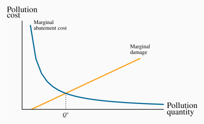
To see how these different policies operate, consider first Figure 5.7. It is a standard diagram in environmental economics, and is somewhat similar to our supply and demand curves. On the horizontal axis is measured the quantity of environmental damage or pollution, and on the vertical axis its dollar value or cost. The upward-sloping damage curve represents the cost to society of each additional unit of pollution or gas, and it is therefore called a marginal damage curve. It is positively sloped to reflect the reality that, at low levels of emissions, the damage of one more unit is less than at higher levels. In terms of our earlier discussion, this means that an increase in GHGs of 10 ppm when concentrations are at 300 ppm may be less damaging than a corresponding increase when concentrations are at 500 ppm.
The marginal damage curve reflects the cost to society of an additional unit of pollution.
The second curve is the abatement curve. It reflects the cost of reducing emissions by one unit, and is therefore called a marginal abatement curve. This curve has a negative slope indicating that, as we reduce the total quantity of pollution produced (moving towards the origin on the horizontal axis), the cost of further unit reductions rises. This shape corresponds to reality. For example, halving the emissions of pollutants and gases from automobiles may be achieved by adding a catalytic converter and reducing the amount of lead in gasoline. But reducing those emissions all the way to zero requires the development of major new technologies such as electric cars—an enormously more costly undertaking.
The marginal abatement curve reflects the cost to society of reducing the quantity of pollution by one unit.
If producers are unconstrained in the amount of pollution they produce, they will produce more than what we will show is the optimal amount – corresponding to Q×. This amount is optimal in the sense that at levels greater than Q× the damage exceeds the cost of reducing the emissions. However, reducing emissions below Q× would mean incurring a cost per unit reduction that exceeds the benefit of that reduction. Another way of illustrating this is to observe that at a level of pollution above Q× the cost of reducing it is less than the damage it inflicts, and therefore a net gain accrues to society as a result of the reduction. But to reduce pollution below Q× would involve an abatement cost greater than the reduction in pollution damage and therefore no net gain to society. This constitutes a first rule in optimal pollution policy.
An optimal quantity of pollution occurs when the marginal cost of abatement equals the marginal damage.
A second guiding principle emerges by considering a situation in which some firms are relatively 'clean' and others are 'dirty'. More specifically, a clean firm A may have already invested in new equipment that uses less energy per unit of output produced, or emits fewer pollutants per unit of output. In contrast, the dirty firm B uses older dirtier technology. Suppose furthermore that these two firms form a particular sector of the economy and that the government sets a limit on total pollution from this sector, and that this limit is less than what the two firms are currently producing. What is the least costly method to meet the target?
The intuitive answer to this question goes as follows: In order to reduce pollution at least cost to the sector, calculate what it would cost each firm to reduce pollution from its present level. Then implement a system so that the firm with the least cost of reduction is the first to act. In this case the 'dirty' firm will likely have a lower cost of abatement since it has not yet upgraded its physical plant. This leads to a second rule in pollution policy:
With many polluters, the least cost policy to society requires producers with the lowest abatement costs to act first.
This principle implies that policies which impose the same emission limits on firms may not be the least costly manner of achieving a target level of pollution. Let us now consider the use of tradable permits and corrective/carbon taxes as policy instruments. These are market-based systems aimed at reducing GHGs.
Tradable permits and corrective/carbon taxes are market-based systems aimed at reducing GHGs.
Incentive mechanism I: Tradable permits
A system of tradable permits is frequently called a 'cap and trade' system, because it limits or caps the total permissible emissions, while at the same time allows a market to develop in permits. For illustrative purposes, consider the hypothetical two-firm sector we developed above, composed of firms A and B. Firm A has invested in clean technology, firm B has not. Thus it is less costly for B to reduce emissions than A if further reductions are required. Next suppose that each firm is allocated by the government a specific number of 'GHG emission permits'; and that the total of such permits is less than the amount of emissions at present, and that each firm is emitting more than its permits allow. How can these firms achieve the target set for this sector of the economy?
The answer is that they should be able to engage in mutually beneficial trade: If firm B has a lower cost of reducing emissions than A, then it may be in A's interest to pay B to reduce B's emissions heavily. Imagine that each firm is emitting 60 units of GHG, but they have permits to emit only 50 units each. And furthermore suppose it costs B $20 to reduce GHGs by one unit, whereas it costs A $30 to do this. In this situation A could pay B $25 for several permits and this would benefit both firms. B can reduce GHGs at a cost of $20 and is being paid $25 to do this. In turn A would incur a cost of $30 per unit to reduce his GHGs but he can buy permits from B for just $25 and avoid the $30 cost. Both firms gain, and the total cost to the economy is lower than if each firm had to reduce by the same amount.
The benefit of the cap 'n trade system is that it enables the marketplace to reduce GHGs at least cost.
The largest system of tradable permits currently operates in the European Union: The EU Emissions Trading System. It covers more than 10,000 large energy-using installations. Trading began in 2005. In North America a number of Western states and several Canadian provinces are joined, either as participants or observers, in the Western Climate Initiative, which is committed to reduce GHGs by means of tradable emissions permits. The longer-term goal of these systems is for the government to issue progressively fewer permits each year, and to include an ever larger share of GHG-emitting enterprises with the passage of time.
Policy in practice – international
In an ideal world, permits would be traded internationally, and such a system might be of benefit to developing economies: If the cost of reducing pollution is relatively low in developing economies because they have few controls in place, then developed economies, for whom the cost of GA reduction is high, could induce firms in the developing world to undertake cost reductions. Such a trade would be mutually beneficial. For example, imagine in the above example that B is located in the developing world and A in the developed world. Both would obviously gain from such an arrangement, and because GHGs are a common property, the source of GHGs from a damage standpoint is immaterial.
Incentive mechanism II: Taxes
Corrective taxes are frequently called Pigovian taxes, after the economist Arthur Pigou. He advocated taxing activities that cause negative externalities. These taxes have been examined above in Section 5.4. Corrective taxes of this type can be implemented as part of a tax package reform. For example, taxpayers are frequently reluctant to see governments take 'yet more' of their money, in the form of new taxes. Such concerns can be addressed by reducing taxes in other sectors of the economy, in such a way that the package of tax changes maintains a 'revenue neutral' impact.
Revenues from taxes and permits
Taxes and tradable permits differ in that taxes generate revenue for the government from polluting producers, whereas permits may not generate revenue, or may generate less revenue. If the government simply allocates permits initially to all polluters, free of charge, and allows a market to develop, such a process generates no revenue to the government. While economists may advocate an auction of permits in the start-up phase of a tradable permits market, such a mechanism may run into political objections.
Setting taxes at the appropriate level requires knowledge of the cost and damage functions associated with GHGs. At the present time, economists and environmental scientists think that an appropriate price or tax on one tonne of GHG is in the  range. Such a tax would reduce emissions to a point where the longer-term impact of GHGs would not be so severe as otherwise.
British Columbia introduced a carbon tax of  per tonne of GHG on fuels in 2008, and has increased that price regularly. This tax was designed to be revenue neutral in order to make it more acceptable. This means that British Columbia reduced its income tax rates by an amount such that income tax payments would fall by an amount equal to the revenue captured by the carbon tax.
GHG policy at the federal level in Canada is embodied in the Greenhouse Gas Pollution Pricing Act of 2018. As detailed earlier, the Act imposes a yearly increasing levy on emissions. The system is intended to be revenue neutral, in that the revenues will be returned to households in the form of a 'paycheck' by the federal government. Large emitters of GHGs are permitted a specific threshold number of tonnes of emission each year without being penalized. Beyond that threshold the above rates apply.
Will this amount of carbon taxation hurt consumers, and will it enable Canada to reach its 2030 GHG goal? As a specific example: the gasoline-pricing rule of thumb is that each in carbon taxation or pricing leads to an increase in the price of gasoline at the pump of about 2.5 cents. So a  levy per tonne means gas at the pump should rise by 12.5 cents per litre. The proceeds are returned to households.
As for the goal of reaching the 2030 target announced at Paris: Environment Canada estimates that the pricing scheme will reduce GHG emissions by about 60 tonnes per annum. But Canada's goal stated in Paris is to reduce emissions in 2030 by approximately four times this amount. Under the Paris Accoord, Canada stated that its 2030 goal would be to reduce emissions by 30% from their 2005 level of 725 MT, that is by an amount equal to approximately 220 tonnes.
Policy in practice – domestic large final emitters
Governments frequently focus upon quantities emitted by individual large firms, or large final emitters (LFEs). In some economies, a relatively small number of producers are responsible for a disproportionate amount of an economy's total pollution, and limits are placed on those firms in the belief that significant economy-wide reductions can be achieved in this manner. One reason for concentrating on these LFEs is that the monitoring costs are relatively small compared to the costs associated with monitoring all firms in the economy. It must be kept in mind that pollution permits may be a legal requirement in some jurisdictions, but monitoring is still required, because firms could choose to risk polluting without owning a permit.