In this chapter we will explore:
| 8.1 | Efficient production
|
| 8.2 | Time frames: The short run and the long run
|
| 8.3 | Production in the short run
|
| 8.4 | Costs in the short run
|
| 8.5 | Fixed costs and sunk costs
|
| 8.6 | Production and costs in the long run
|
| 8.7 | Technological change and globalization
|
| 8.8 | Clusters, externalities, learning by doing, and scope economies
|
8.1 Efficient production
Firms that fail to operate efficiently seldom survive. They are dominated by
their competitors because the latter produce more efficiently and can sell
at a lower price. The drive for profitability is everywhere present in the
modern economy. Companies that promise more profit, by being more efficient,
are valued more highly on the stock exchange. For example: In July of 2015
Google announced that, going forward, it would be more attentive to cost
management in its numerous research endeavours that aim to bring new
products to the marketplace. This policy, put in place by the Company's new
Chief Financial Officer, was welcomed by investors who, as a result, bought
up the stock. The Company's stock increased in value by 16% in one day – equivalent
to about $50 billion.
The remuneration of managers in virtually all corporations is linked to
profitability. Efficient production, a.k.a. cost reduction, is
critical to achieving this goal. In this chapter we will examine cost
management and efficient production from the ground up – by exploring how a
small entrepreneur brings his or her product to market in the most efficient
way possible. As we shall see, efficient production and cost minimization
amount to the same thing: Cost minimization is the financial reflection of
efficient production.
Efficient production is critical in any budget-driven organization, not just
in the private sector. Public institutions equally are, and should be,
concerned with costs and efficiency.
Entrepreneurs employ factors of production (capital and labour) in order to
transform raw materials and other inputs into goods or services. The
relationship between output and the inputs used in the production process is
called a production function. It specifies how much output can
be produced with given combinations of inputs. A production function is not
restricted to profit-driven organizations. Municipal road repairs are
carried out with labour and capital. Students are educated with teachers,
classrooms, computers, and books. Each of these is a production process.
Production function: a technological relationship that specifies how much output can be produced with specific amounts of inputs.
Economists distinguish between two concepts of efficiency: One is technological efficiency;
the other is economic efficiency. To illustrate
the difference, consider the case of auto assembly: the assembler could produce its vehicles either by
using a large number of assembly workers and a plant that has a relatively
small amount of machinery, or it could use fewer workers accompanied by more
machinery in the form of robots. Each of these processes could be deemed
technologically efficient, provided that there is no waste. If the workers
without robots are combined with their capital to produce as much as
possible, then that production process is technologically efficient.
Likewise, in the scenario with robots, if the workers and capital are
producing as much as possible, then that process too is efficient in the
technological sense.
Technological efficiency means that the maximum output is produced with the given set of inputs.
Economic efficiency is concerned with more than just technological
efficiency. Since the entrepreneur's goal is to make profit, she must
consider which technologically efficient process best achieves that
objective. More broadly, any budget-driven process should focus on being
economically efficient, whether in the public or private sector. An
economically efficient production structure is the one that produces output
at least cost.
Economic efficiency defines a production structure that produces output at least cost.
Auto-assembly plants the world over have moved to using robots during the
last two decades. Why? The reason is not that robots were invented 20 years
ago; they were invented long before that. The real reason is that, until
recently, this technology was not economically efficient. Robots were too
expensive; they were not capable of high-precision assembly. But once their
cost declined and their accuracy increased they became economically
efficient. The development of robots represented technological progress.
When this progress reached a critical point, entrepreneurs embraced it.
To illustrate the point further, consider the case of garment assembly.
There is no doubt that engineers could make robots capable of joining
the pieces of fabric that form garments. This is not beyond our
technological abilities. Why, then, do we not have such capital-intensive
production processes for garment making, similar to the production process
chosen by vehicle producers? The answer is that, while such a concept could
be technologically efficient, it would not be economically efficient. It is
more profitable to use large amounts of labour and relatively traditional
machines to assemble garments, particularly when labour in Asia costs less and
the garments can be shipped back to Canada inexpensively. Containerization and scale economies in shipping mean that a
garment can be shipped to Canada from Asia for a few cents per unit.
Efficiency in production is not limited to the manufacturing sector. Farmers
must choose the optimal combination of labour, capital and fertilizer to
use. In the health and education sectors, efficient supply involves choices
on how many high- and low-skill workers to employ, how much traditional
physical capital to use, how much information technology to use, based upon
the productivity and cost of each. Professors and physicians are costly
inputs. When they work with new technology (capital) they become more
efficient at performing their tasks: It is less costly to have a single
professor teach in a 300-seat classroom that is equipped with the latest
technology, than have several professors each teaching 60-seat classes with
chalk and a blackboard.
8.2 The time frame
We distinguish initially between the short run and the
long run. When discussing technological change, we use the
term very long run. These concepts have little to do with
clocks or calendars; rather, they are defined by the degree of flexibility
an entrepreneur or manager has in her production process. A key decision
variable is capital.
A customary assumption is that a producer can hire more labour immediately,
if necessary, either by taking on new workers (since there are usually some
who are unemployed and looking for work), or by getting the existing workers
to work longer hours. In contrast, getting new capital in place is usually
more time consuming: The entrepreneur may have to place an order for new
machinery, which will involve a production and delivery time lag. Or she may
have to move to a more spacious location in order to accommodate the added
capital. Whether this calendar time is one week, one month, or one year is
of no concern to us. We define the long run as a period of sufficient length
to enable the entrepreneur to adjust her capital stock, whereas in the short
run at least one factor of production is fixed. Note that it matters little
whether it is labour or capital that is fixed in the short run. A software
development company may be able to install new capital (computing power)
instantaneously but have to train new developers. In such a case capital is
variable and labour is fixed in the short run. The definition of the short
run is that one of the factors is fixed, and in our examples we will assume
that it is capital.
Short run: a period during which at least one factor of production is fixed. If capital is fixed, then more output is produced by using additional labour.
Long run: a period of time that is sufficient to enable all factors of production to be adjusted.
Very long run: a period sufficiently long for new technology to develop.
8.3 Production in the short run
Black Diamond Snowboards (BDS) is a start-up snowboard producing enterprise.
Its founder has invented a new lamination process that gives extra strength
to his boards. He has set up a production line in his garage that has four
workstations: Laminating, attaching the steel edge, waxing, and packing.
With this process in place, he must examine how productive his firm can be.
After extensive testing, he has determined exactly how his productivity
depends upon the number of workers. If he employs only one worker, then that
worker must perform several tasks, and will encounter 'down time' between
workstations. Extra workers would therefore not only increase the total
output; they could, in addition, increase output per worker. He
also realizes that once he has employed a critical number of workers,
additional workers may not be so productive: Because they will have to share
the fixed amount of machinery in his garage, they may have to wait for
another worker to finish using a machine. At such a point, the productivity
of his plant will begin to fall off, and he may want to consider capital
expansion. But for the moment he is constrained to using this particular
assembly plant. Testing leads him to formulate the relationship between
workers and output that is described in Table 8.1.
Table 8.1 Snowboard production and productivity
|
1 | 2 | 3 | 4 | 5 |
|
Workers | Output | Marginal | Average | Stages of |
|
| (TP) | product | product | production |
|
| | (MPL) | (APL) | |
|
0 | 0 | | | MPL increasing |
|
1 | 15 | 15 | 15 |
|
2 | 40 | 25 | 20 |
|
3 | 70 | 30 | 23.3 |
|
4 | 110 | 40 | 27.5 |
|
5 | 145 | 35 | 29 | MPL positive and declining |
|
6 | 175 | 30 | 29.2 |
|
7 | 200 | 25 | 28.6 |
|
8 | 220 | 20 | 27.5 |
|
9 | 235 | 15 | 26.1 |
|
10 | 240 | 5 | 24.0 |
|
11 | 235 | -5 | 21.4 | MPL negative |
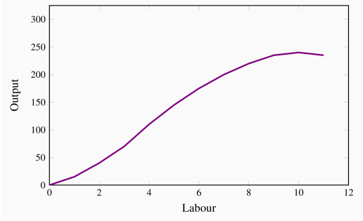
By increasing the number of workers in the plant, BDS produces more boards.
The relationship between these two variables in columns 1 and 2 in the table
is plotted in Figure 8.1. This is called the
total product function (TP), and it defines the output
produced with different amounts of labour in a plant of fixed size.
Total product is the relationship between total output produced and the number of workers employed, for a given amount of capital.
This relationship is positive, indicating that more workers produce more
boards. But the curve has an interesting pattern. In the initial expansion
of employment it becomes progressively steeper – its curvature is slightly
convex; following this phase the function's increase becomes progressively
less steep – its curvature is concave. These different stages in the TP
curve tell us a great deal about productivity in BDS. To see this, consider
the additional number of boards produced by each worker. The first worker
produces 15. When a second worker is hired, the total product rises to 40,
so the additional product attributable to the second worker is 25. A third
worker increases output by 30 units, and so on. We refer to this additional
output as the marginal product (MP) of an additional worker, because it
defines the incremental, or marginal, contribution of the worker. These
values are entered in column 3.
More generally the MP of labour is defined as the change in output divided
by the change in the number of units of labour employed. Using, as before,
the Greek capital delta ( ) to denote a change, we can define
In this example the change in labour is one unit at each stage and hence the marginal product of labour is simply the corresponding change
in output. It is also the case that the MPL is the slope of the TP
curve – the change in the value on the vertical axis due to a change in the
value of the variable on the horizontal axis.
Marginal product of labour is the addition to output produced by each additional worker. It is also the slope of the total product curve.
During the initial stage of production expansion, the marginal product of
each worker is increasing. It increases from 15 to 40 as BDS moves from
having one employee to four employees. This increasing MP is made possible
by the fact that each worker is able to spend more time at his workstation,
and less time moving between tasks. But, at a certain point in the
employment expansion, the MP reaches a maximum and then begins to tail
off. At this stage – in the concave region of the TP curve – additional
workers continue to produce additional output, but at a diminishing rate.
For example, while the fourth worker adds 40 units to output, the fifth
worker adds 35, the sixth worker 30, and so on. This declining MP is due
to the constraint of a fixed number of machines: All workers must share the
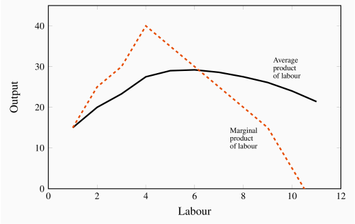
same capital. The MP function is plotted in Figure 8.2.
The phenomenon we have just described has the status of a law in economics:
The law of diminishing returns states that, in the face of a
fixed amount of capital, the contribution of additional units of a variable
factor must eventually decline.
Law of diminishing returns: when increments of a variable factor (labour) are added to a fixed amount of another factor (capital), the marginal product of the variable factor must eventually decline.
The relationship between Figures 8.1 and 8.2
should be noted. First, the MPL reaches a maximum at an output of 4 units
– where the slope of the TP curve is greatest. The MPL curve remains
positive beyond this output, but declines: The TP curve reaches a maximum
when the tenth unit of labour is employed. An eleventh unit actually reduces
total output; therefore, the MP of this eleventh worker is negative! In
Figure 8.2, the MP curve becomes negative at this point.
The garage is now so crowded with workers that they are beginning to
obstruct the operation of the production process. Thus the producer would
never employ an eleventh unit of labour.
Next, consider the information in the fourth column of the table. It defines
the average product of labour (APL)—the amount of output produced, on
average, by workers at different employment levels:
This function is also plotted in Figure 8.2. Referring to the
table: The AP column indicates, for example, that when two units of labour
are employed and forty units of output are produced, the average production
level of each worker is 20 units (=40/2). When three workers produce 70
units, their average production is 23.3 (=70/3), and so forth. Like the MP
function, this one also increases and subsequently decreases, reflecting
exactly the same productivity forces that are at work on the MP curve.
Average product of labour is the number of units of output produced per unit of labour at different levels of employment.
The AP and MP functions intersect at the point where the AP is at its
peak. This is no accident, and has a simple explanation. Imagine a softball
player who is batting .280 coming into today's game—she has been hitting
her way onto base 28 percent of the time when batting, so far this
season. This is her average product, AP.
In today's game, if she bats .500 (hits her way to base on half of her
at-bats), then she will improve her average. Today's batting (MP) at
.500 therefore pulls up the season's AP. Accordingly, whenever the MP
exceeds the AP, the AP is pulled up. By the same reasoning, if her MP
is less than the season average, her average will be pulled down. It follows
that the two functions must intersect at the peak of the AP curve. To
summarize:
If the MP exceeds the AP, then the AP increases;
If the MP is less than the AP, then the AP declines.
While the owner of BDS may understand his productivity relations, his
ultimate goal is to make profit, and for this he must figure out how
productivity translates into cost.
8.4 Costs in the short run
The cost structure for the production of snowboards at Black Diamond is
illustrated in Table 8.2. Employees are skilled and are
paid a weekly wage of $1,000. The cost of capital is $3,000 and it is
fixed, which means that it does not vary with output. As in Table 8.1, the number of employees and the output are given in the
first two columns. The following three columns define the capital costs, the
labour costs, and the sum of these in producing different levels of output.
We use the terms fixed, variable, and total costs to define the cost structure of a firm. Fixed
costs do not vary with output, whereas variable costs do, and total costs
are the sum of fixed and variable costs. To keep this example as simple as
possible, we will ignore the cost of raw materials. We could add an
additional column of costs, but doing so will not change the conclusions.
Table 8.2 Snowboard production costs
|
Workers | Output | Capital | Labour | Total | Average | Average | Average | Marginal |
|
| | cost | cost | costs | fixed | variable | total | cost |
|
| | fixed | variable | | cost | cost | cost | |
|
0 | 0 | 3,000 | 0 | 3,000 | | | | |
|
1 | 15 | 3,000 | 1,000 | 4,000 | 200.0 | 66.7 | 266.7 | 66.7 |
|
2 | 40 | 3,000 | 2,000 | 5,000 | 75.0 | 50.0 | 125.0 | 40.0 |
|
3 | 70 | 3,000 | 3,000 | 6,000 | 42.9 | 42.9 | 85.7 | 33.3 |
|
4 | 110 | 3,000 | 4,000 | 7,000 | 27.3 | 36.4 | 63.6 | 25.0 |
|
5 | 145 | 3,000 | 5,000 | 8,000 | 20.7 | 34.5 | 55.2 | 28.6 |
|
6 | 175 | 3,000 | 6,000 | 9,000 | 17.1 | 34.3 | 51.4 | 33.3 |
|
7 | 200 | 3,000 | 7,000 | 10,000 | 15.0 | 35.0 | 50.0 | 40.0 |
|
8 | 220 | 3,000 | 8,000 | 11,000 | 13.6 | 36.4 | 50.0 | 50.0 |
|
9 | 235 | 3,000 | 9,000 | 12,000 | 12.8 | 38.3 | 51.1 | 66.7 |
|
10 | 240 | 3,000 | 10,000 | 13,000 | 12.5 | 41.7 | 54.2 | 200.0 |
Fixed costs are costs that are independent of the level of output.
Variable costs are related to the output produced.
Total cost is the sum of fixed cost and variable cost.
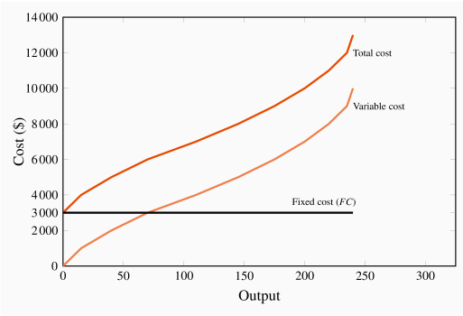
Total costs are illustrated in Figure 8.3 as the vertical sum
of variable and fixed costs. For example, Table 8.2
indicates that the total cost of producing 220 units of output is the sum of
$3,000 in fixed costs plus $8,000 in variable costs. Therefore, at the
output level 220 on the horizontal axis in Figure 8.3, the sum
of the cost components yields a value of $11,000 that forms one point on
the total cost curve. Performing a similar calculation for every possible
output yields a series of points that together form the complete total cost
curve.
Average costs are given in the next three columns of Table 8.2. Average cost is the cost per unit of output, and we
can define an average cost corresponding to each of the fixed, variable, and
total costs defined above. Average fixed cost (AFC) is the
total fixed cost divided by output; average variable cost (AVC) is the total variable cost divided by output; and average
total cost (ATC) is the total cost divided by output.
|
AFC |  |
|
AVC |  |
|
ATC | =AFC+AVC
|
Average fixed cost is the total fixed cost per unit of output.
Average variable cost is the total variable cost per unit of output.
Average total cost is the sum of all costs per unit of output.
The productivity-cost relationship
Consider the average variable cost - average product relationship,
as developed in column 7 of Table 8.2; its
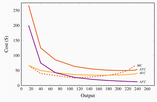
corresponding variable cost curve is plotted in Figure 8.4.
In this example, AVC first decreases and then increases. The intuition
behind its shape is straightforward (and realistic) if you have understood
why productivity varies in the short run: The variable cost, which
represents the cost of labour, is constant per unit of labour, because the
wage paid to each worker does not change. However, each worker's
productivity varies. Initially, when we hire more workers, they become more
productive, perhaps because they have less 'down time' in switching between
tasks. This means that the labour costs per snowboard must decline. At some
point, however, the law of diminishing returns sets in: As before, each
additional worker is paid a constant amount, but as productivity declines
the labour cost per snowboard increases.
In this numerical example the AP is at a maximum when six units of labour
are employed and output is 175. This is also the point where the AVC is at
a minimum. This maximum/minimum relationship is also illustrated in Figures 8.2 and 8.4.
Now consider the marginal cost - marginal product relationship. The marginal cost (MC) defines the cost of producing one more
unit of output. In Table 8.2, the marginal cost of
output is given in the final column. It is the additional cost of production
divided by the additional number of units produced. For example, in going
from 15 units of output to 40, total costs increase from $4,000 to $5,000.
The MC is the cost of those additional units divided by the number of
additional units. In this range of output, MC is  . We
could also calculate the MC as the addition to variable costs rather than
the addition to total costs, because the addition to each is the
same—fixed costs are fixed. Hence:
. We
could also calculate the MC as the addition to variable costs rather than
the addition to total costs, because the addition to each is the
same—fixed costs are fixed. Hence:
|
MC |  |
|
|  |
Marginal cost of production is the cost of producing each additional unit of output.
Just as the behaviour of the AVC curve is determined by the AP curve, so
too the behaviour of the MC is determined by the MP curve. When the MP
of an additional worker exceeds the MP of the previous worker, this
implies that the cost of the additional output produced by the last worker
hired must be declining. To summarize:
If the marginal product of labour increases, then the marginal cost of
output declines;
If the marginal product of labour declines, then the marginal cost of output
increases.
In our example, the  reaches a maximum when the fourth unit of
labour is employed (or 110 units of output are produced), and this also is
where the MC is at a minimum. This illustrates that the marginal
cost reaches a minimum at the output level where the marginal product
reaches a maximum.
reaches a maximum when the fourth unit of
labour is employed (or 110 units of output are produced), and this also is
where the MC is at a minimum. This illustrates that the marginal
cost reaches a minimum at the output level where the marginal product
reaches a maximum.
The average total cost is the sum of the fixed cost per unit of output and
the variable cost per unit of output. Typically, fixed costs are the
dominant component of total costs at low output levels, but become less
dominant at higher output levels. Unlike average variable costs, note that
the average fixed cost must always decline with output, because a fixed cost
is being spread over more units of output. Hence, when the ATC curve
eventually increases, it is because the increasing variable cost component
eventually dominates the declining AFC component. In our example, this
occurs when output increases from 220 units (8 workers) to 235 (9 workers).
Finally, observe the interrelationship between the MC curve on the one
hand and the ATC and AVC on the other. Note from Figure 8.4 that the MC cuts the AVC and the ATC at the minimum
point of each of the latter. The logic behind this pattern is analogous to
the logic of the relationship between marginal and average product curves:
When the cost of an additional unit of output is less than the average, this
reduces the average cost; whereas, if the cost of an additional unit of
output is above the average, this raises the average cost. This must hold
true regardless of whether we relate the MC to the ATC or the AVC.
When the marginal cost is less than the average cost, the average cost must
decline;
When the marginal cost exceeds the average cost, the average cost must
increase.
Notation: We use both the abbreviations  and
and
 to denote average total cost. The term 'average
cost' is understood in economics to include both fixed and variable costs.
to denote average total cost. The term 'average
cost' is understood in economics to include both fixed and variable costs.
Teams and services
The choice faced by the producer in the example above is slightly
'stylized', yet it still provides an appropriate rule for analyzing hiring
decisions. In practice, it is quite difficult to isolate or identify the
marginal product of an individual worker. One reason is that individuals
work in teams within organizations. The accounting department, the marketing
department, the sales department, the assembly unit, the chief executive's
unit are all composed of teams. Adding one more person to human resources
may have no impact on the number of units of output produced by the company
in a measurable way, but it may influence worker morale and hence
longer-term productivity. Nonetheless, if we consider expanding, or
contracting, any one department within an organization, management can
attempt to estimate the net impact of additional hires (or layoffs) on the
contribution of each team to the firm's profitability. Adding a person in
marketing may increase sales, laying off a person in research and
development may reduce costs by more than it reduces future value to the
firm. In practice this is what firms do: they attempt to assess the
contribution of each team in their organization to costs and revenues, and
on that basis determine the appropriate number of employees.
The manufacturing sector of the macro economy is dominated, sizewise, by the
services sector. But the logic that drives hiring decisions, as developed
above, applies equally to services. For example, how does a law firm
determine the optimal number of paralegals to employ per lawyer? How many
nurses are required to support a surgeon? How many university professors are
required to teach a given number of students?
All of these employment decisions involve optimization at the margin. The
goal of the decision maker is not always profit, but she should attempt to
estimate the cost and value of adding personnel at the margin.
8.5 Fixed costs and sunk costs
The distinction between fixed and variable costs is important for producers
who are not making a profit. If a producer has committed
himself to setting up a plant, then he has made a decision to incur a fixed
cost. Having done this, he must now decide on a production strategy that
will maximize profit. However, the price that consumers are willing to pay
may not be sufficient to yield a profit. So, if Black Diamond Snowboards
cannot make a profit, should it shut down? The answer is that if it can
cover its variable costs, having already incurred its fixed costs,
it should stay in production, at least temporarily. By covering the variable
cost of its operation, Black Diamond is at least earning some return. A
sunk cost is a fixed cost that has already been incurred and
cannot be recovered. But if the pressures of the marketplace are so great
that the total costs cannot be covered in the longer run, then this is not a
profitable business and the firm should close its doors.
Is a fixed cost always a sunk cost? No: Any production that involves capital
will incur a fixed cost component. Such
capital can be financed in several ways however: It might be financed on a
very short-term lease basis, or it might have been purchased by the
entrepreneur. If it is leased on a month-to-month basis, an unprofitable
entrepreneur who can only cover variable costs (and who does not foresee
better market conditions ahead) can exit the industry quickly – by not
renewing the lease on the capital. But an individual who has actually
purchased equipment that cannot readily be resold has essentially sunk money
into the fixed cost component of his production. This entrepreneur should
continue to produce as long as he can cover variable costs.
Sunk cost is a fixed cost that has already been incurred and cannot be recovered, even by producing a zero output.
R & D as a sunk cost
Sunk costs in the modern era are frequently in the form of research and
development costs, not the cost of building a plant or purchasing machinery.
The prototypical example is the pharmaceutical industry, where it is
becoming progressively more challenging to make new drug breakthroughs –
both because the 'easier' breakthroughs have already been made, and because
it is necessary to meet tighter safety conditions attaching to new drugs.
Research frequently leads to drugs that are not sufficiently effective in
meeting their target. As a consequence, the pharmaceutical sector regularly
writes off hundreds of millions of dollars of lost sunk costs – unfruitful
research and development.
Finally, we need to keep in mind the opportunity costs of running the
business. The owner pays himself a salary, and ultimately he must recognize
that the survival of the business should not depend upon his drawing a
salary that is less than his opportunity cost. As developed in Section 7.2, if he underpays himself in
order to avoid shutting down, he might be better off in the long run to
close the business and earn his opportunity cost elsewhere in the
marketplace.
A dynamic setting
We need to ask why it might be possible to cover all costs in a longer run horizon, while in the near-term costs are not covered. The principal reason is that demand may grow, particularly for a new product. For example, in 2019 numerous cannabis producing firms were listed on the Canadian Securities Exchange, and collectively were valued at about fifty billion dollars. None had revenues that covered costs, yet investors poured money into this sector. Investors evidently envisaged that the market for legal cannabis would grow. As of 2020 it appears that these investors were excessively optimistic. Sales growth has been slow and stock valuations have plummeted.
8.6 Long-run production and costs
The snowboard manufacturer we portray produces a relatively low level of
output; in reality, millions of snowboards are produced each year in the
global market. Black Diamond Snowboards may have hoped to get a start by
going after a local market—the "free-ride" teenagers at Mont Sainte Anne
in Quebec or at Fernie in British Columbia. If this business takes off, the
owner must increase production, take the business out of his garage and set
up a larger-scale operation. But how will this affect his cost structure?
Will he be able to produce boards at a lower cost than when he was producing
a very limited number of boards each season? Real-world experience would
indicate yes.
Production costs almost always decline when the scale of the
operation initially increases. We refer to this phenomenon simply as economies of scale. There are several reasons why scale
economies are encountered. One is that production flows can be organized in
a more efficient manner when more is being produced. Another is that the
opportunity to make greater use of task specialization presents itself; for
example, Black Diamond Snowboards may be able to subdivide tasks within the
laminating and packaging stations. With a larger operating scale the replacement of labor with capital may be economically efficient. If scale economies do define the real
world, then a bigger plant—one that is geared to produce a higher level of
output—should have an average total cost curve that is "lower" than the
cost curve corresponding to the smaller scale of operation we considered in
the example above.
Average costs in the long run
Figure 8.5 illustrates a possible relationship between
the ATC curves for four different scales of operation.  is the
average total cost curve associated with a small-sized plant; think of it as
the plant built in the entrepreneur's garage.
is the
average total cost curve associated with a small-sized plant; think of it as
the plant built in the entrepreneur's garage.  is associated with a
somewhat larger plant, perhaps one she has put together in a rented
industrial or commercial space. The further a cost curve is located to the
right of the diagram the larger the production facility it defines, given
that output is measured on the horizontal axis. If there are economies
associated with a larger scale of operation, then the average costs
associated with producing larger outputs in a larger plant should be lower
than the average costs associated with lower outputs in a smaller plant,
assuming that the plants are producing the output levels they were designed
to produce. For this reason, the cost curve and the cost curve
is associated with a
somewhat larger plant, perhaps one she has put together in a rented
industrial or commercial space. The further a cost curve is located to the
right of the diagram the larger the production facility it defines, given
that output is measured on the horizontal axis. If there are economies
associated with a larger scale of operation, then the average costs
associated with producing larger outputs in a larger plant should be lower
than the average costs associated with lower outputs in a smaller plant,
assuming that the plants are producing the output levels they were designed
to produce. For this reason, the cost curve and the cost curve
 each have a segment that is lower than the lowest segment on
. However, in Figure 8.5 the cost curve
each have a segment that is lower than the lowest segment on
. However, in Figure 8.5 the cost curve  has moved upwards. What behaviours are implied here?
In many production environments, beyond some large scale of operation, it
becomes increasingly difficult to reap further cost reductions from
specialization, organizational economies, or marketing economies. At such a
point, the scale economies are effectively exhausted, and larger plant sizes
no longer give rise to lower (short-run) ATC curves. This is reflected in the
similarity of the and the curves. The pattern suggests
that we have almost exhausted the possibilities of further scale advantages once we
build a plant size corresponding to . Consider next what is implied by the
position of the curve relative to the and
curves. The relatively higher position of the curve implies that
unit costs will be higher in a yet larger plant. Stated differently: If we
increase the scale of this firm to extremely high output levels, we are
actually encountering diseconomies of scale. Diseconomies of
scale imply that unit costs increase as a result of the firm's becoming too
large: Perhaps co-ordination difficulties have set in at the very high
output levels, or quality-control monitoring costs have risen. These
coordination and management difficulties are reflected in increasing unit
costs in the long run.
The terms increasing, constant, and
decreasing returns to scale underlie the concepts of scale
economies and diseconomies: Increasing returns to scale (IRS) implies that,
when all inputs are increased by a given proportion, output increases more
than proportionately. Constant returns to scale (CRS) implies that output
increases in direct proportion to an equal proportionate increase in all
inputs. Decreasing returns to scale (DRS) implies that an equal
proportionate increase in all inputs leads to a less than proportionate
increase in output.
Increasing returns to scale implies that, when all inputs are increased by a given proportion, output increases more than proportionately.
Constant returns to scale implies that output increases in direct proportion to an equal proportionate increase in all inputs.
Decreasing returns to scale implies that an equal proportionate increase in all inputs leads to a less than proportionate increase in output.
These are pure production function relationships, but, if the prices of
inputs are fixed for producers, they translate directly into the various
cost structures illustrated in Figure 8.5. For example,
if a 40% increase in capital and labour use allows for better production
flows than when in the smaller plant, and therefore yields more than a 40%
increase in output, this implies that the cost per snowboard produced must
fall in the new plant. In contrast, if a 40% increase in capital and labour
leads to say just a 30% increase in output, then the cost per snowboard in
the new larger plant must be higher. Between these extremes, there may be a
range of relatively constant unit costs, corresponding to where the
production relation is subject to constant returns to scale. In
Figure 8.5, the falling unit costs output region has increasing
returns to scale, the region that has relatively constant unit costs has
constant returns to scale, and the increasing cost region has decreasing
returns to scale.
Increasing returns to scale characterize businesses with large initial costs
and relatively low costs of producing each unit of output. Computer chip
manufacturers, pharmaceutical manufacturers, vehicle rental agencies, booking agencies such as booking.com or hotels.com, intermediaries such as airbnb.com, even brewers, all benefit from scale economies. In the beer market, brewing, bottling and
shipping are all low-cost operations relative to the capital cost of setting
up a brewery. Consequently, we observe surprisingly few breweries in any
brewing company, even in large land-mass economies such as Canada or the US.
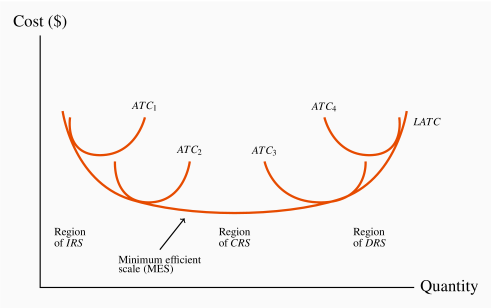
In addition to the four short-run average total cost curves, Figure 8.5
contains a curve that forms an envelope around the bottom
of these short-run average cost curves. This envelope is the
long-run average total cost (LATC) curve, because it defines
average cost as we move from one plant size to another. Remember that in the
long run both labour and capital are variable, and as we move from one
short-run average cost curve to another, that is exactly what happens—all
factors of production are variable. Hence, the collection of short-run cost
curves in Figure 8.5 provides the ingredients for a
long-run average total cost curve.
Long-run average total cost is the lower envelope of all the short-run ATC curves.
The particular range of output on the LATC where it begins to flatten out is
called the range of minimum efficient scale. This is an
important concept in industrial policy, as we shall see in later chapters.
At such an output level, the producer has expanded sufficiently to take
advantage of virtually all the scale economies available.
Minimum efficient scale defines a threshold size of operation such that scale
economies are almost exhausted.
In view of this discussion and the shape of the LATC in
Figure 8.5, it is obvious that economies of scale can also be
defined in terms of the curvature of the LATC. Where the LATC declines
there are IRS, where the LATC is flat there are CRS, where the LATC
slopes upward there are DRS.
Table 8.3 LATC elements for two plants (thousands $)
| Q |  |  | |  |  | |
|
20 | 50 | 30 | 80 | 100 | 25 | 125 |
|
40 | 25 | 30 | 55 | 50 | 25 | 75 |
|
60 | 16.67 | 30 | 46.67 | 33.33 | 25 | 58.33 |
|
80 | 12.5 | 30 | 42.5 | 25 | 25 | 50 |
|
100 | 10 | 30 | 40 | 20 | 25 | 45 |
|
120 | 8.33 | 30 | 38.33 | 16.67 | 25 | 41.67 |
|
140 | 7.14 | 30 | 37.14 | 14.29 | 25 | 39.29 |
|
160 | 6.25 | 30 | 36.25 | 12.5 | 25 | 37.5 |
|
180 | 5.56 | 30 | 35.56 | 11.11 | 25 | 36.11 |
|
200 | 5 | 30 | 35 | 10 | 25 | 35 |
|
220 | 4.55 | 30 | 34.55 | 9.09 | 25 | 34.09 |
|
240 | 4.17 | 30 | 34.17 | 8.33 | 25 | 33.33 |
|
260 | 3.85 | 30 | 33.85 | 7.69 | 25 | 32.69 |
|
280 | 3.57 | 30 | 33.57 | 7.14 | 25 | 32.14 |
Plant 1

m. Plant 2

m. For
Q<200,

; for
Q>200,

; and for
Q=200,
ATC1=
ATC2.
LATC defined by data in bold font.
Long-run costs – a simple numerical example
Kitt is an automobile designer specializing in the production of off-road
vehicles sold to a small clientele. He has a choice of two (and only two)
plant sizes; one involving mainly labour and the other employing robots
extensively. The set-up (i.e. fixed) costs of these two assembly
plants are $1 million and $2 million respectively. The advantage to having
the more costly plant is that the pure production costs (variable costs) are
less. The cost components are defined in Table 8.3. The variable cost (equal
to the marginal cost here) is $30,000 in the plant that relies primarily on
labour, and $25,000 in the plant that has robots. The ATC for each plant
size is the sum of AFC and AVC. The AFC declines as the fixed cost is
spread over more units produced. The variable cost per unit is constant in
each case. By comparing the fourth and final columns, it is clear
that the robot-intensive plant has lower costs if it produces a large number of
vehicles. At an output of 200 vehicles the average costs in each plant are
identical: The higher fixed costs associated with the robots are exactly
offset by the lower variable costs at this output level.
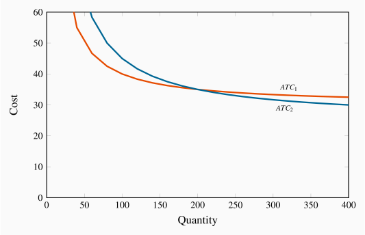
The ATC curve corresponding to each plant size is given in
Figure 8.6. There are two short-run ATC
curves. The positions of these curves indicate that if the manufacturer
believes he can produce at least 200 vehicles his unit costs will be less
with the plant involving robots; but at output levels less than this his
unit costs would be less in the labour-intensive plant.
The long-run average cost curve for this producer is the lower envelope of
these two cost curves: ATC1 up to output 200 and ATC2 thereafter.
Two features of this example are to be noted. First we do not encounter
decreasing returns – the LATC curve never increases. ATC1 tends asymptotically to a lower bound of  , while ATC2 tends towards
  . Second, in the
interests of simplicity we have assumed just two plant sizes are possible.
With more possibilities on the introduction of robots we could imagine more
short-run ATC curves which would form the lower-envelope LATC.
. Second, in the
interests of simplicity we have assumed just two plant sizes are possible.
With more possibilities on the introduction of robots we could imagine more
short-run ATC curves which would form the lower-envelope LATC.
8.7 Technological change: globalization and localization
Technological change represents innovation that can reduce the
cost of production or bring new products on line. As stated earlier, the
very long run is a period that is sufficiently long for new technology to
evolve and be implemented.
Technological change represents innovation that can reduce the cost of production or bring new products on line.
Technological change has had an enormous impact on economic life for several
centuries. It is not something that is defined in terms of the recent
telecommunications revolution. The industrial revolution began in eighteenth
century Britain. It was accompanied by a less well-recognized, but equally
important, agricultural revolution. The improvement in cultivation
technology, and ensuing higher yields, freed up enough labour to populate
the factories that were the core of the industrial revolution. The
development and spread of mechanical power dominated the nineteenth century,
and the mass production line of Henry Ford in autos or Andrew Carnegie in steel heralded in the twentieth century.
Globalization
The modern communications revolution has reduced costs, just like its
predecessors. But it has also greatly sped up globalization,
the increasing integration of national markets.
Globalization is the tendency for international markets to be ever more integrated.
Globalization has several drivers: lower transportation and communication costs; reduced barriers to trade and
capital mobility; the spread of new technologies that facilitate cost
and quality control; different wage rates between developed and less developed economies. New technology and better communications have been
critical in both increasing the minimum efficient scale of operation and
reducing diseconomies of scale; they facilitate the efficient management of
large companies.
The continued reduction in trade barriers in the post-World War II era has
also meant that the effective marketplace has become the globe rather than
the national economy for many products. Companies like Apple, Microsoft, and
Facebook are visible worldwide. Globalization has been accompanied by the
collapse of the Soviet Union, the adoption of an outward looking philosophy
on the part of China, and an increasing role for the market place in India.
These developments together have facilitated the outsourcing of much of the
West's manufacturing to lower-wage economies.
But new technology not only helps existing companies grow large; it also
enables new ones to start up. It is now cheaper for small producers to
manage their inventories and maintain contact with their own suppliers.
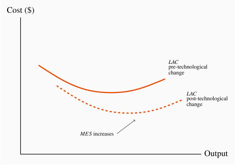
The impact of technology is to reduce the cost of production, hence it will
lower the average cost curve in both the short and long run. First,
decreasing returns to scale become less probable due to improved
communications, so the upward sloping section of the LRAC curve may
disappear altogether. Second, capital costs are now lower than in earlier
times, because much modern technology has transformed some fixed costs into
variable cost: Both software and hardware functions can be subcontracted to
specialty firms, who in turn may use cloud computing services, and it is thus no longer necessary to have a substantial
in-house computing department. The use of almost-free software such as
Skype, Hangouts and WhatsApp reduces
communication costs. Advertising on social media is more effective and less
costly than in traditional hard-print form. Hiring may be cheaper through
LinkedIn than through a traditional human resources department.
These developments may actually reduce the minimum efficient scale of
operation because they reduce the need for large outlays on fixed capital.
On the other hand, changes in technology may induce producers to use more
capital and less labor, with the passage of time. That would increase the
minimum efficient scale. An example of this phenomenon is in mining, or
tunnel drilling, where capital investment per worker is greater than when
technology was less developed. A further example is the introduction of
robotic assistants in Amazon warehouses. In these scenarios the
minimum efficient scale should increase, and that is illustrated in Figure
8.7.
The local diffusion of technology
The impacts of technological change are not just evident in a global
context. Technological change impacts every sector of the domestic economy.
For example, the modern era in dentistry sees specialists in root canals
(endodentists) performing root canals in the space of a single hour with the
help of new technology; dental implants into bone, as an alternative to
dentures, are commonplace; crowns can be machined with little human
intervention; and X-rays are now performed with about one hundredth of the
power formerly required. These technologies spread and are adopted through
several channels. Dental practices do not usually compete on the basis of
price, but if they do not adopt best practices and new technologies, then
community word of mouth will see patients shifting to more efficient
operators.
Some technological developments are protected by patents. But patent
protection rarely inhibits new and more efficient practices that in some way
mimic patent breakthroughs.
8.8 Clusters, learning by doing, scope economies
Clusters
The phenomenon of a grouping of firms that specialize in producing related
products is called a cluster. For example, Ottawa has more
than its share of software development firms; Montreal has a
disproportionate share of Canada's pharmaceutical producers and electronic
game developers; Calgary has its 'oil patch'; Hollywood has movies; Toronto
is Canada's financial capital, San Francisco and Seattle are leaders in new electronic products. Provincial and state capitals have most of
their province's bureaucracy. Clusters give rise to externalities,
frequently in the form of ideas that flow between firms, which in turn
result in cost reductions and new products.
Cluster: a group of firms producing similar products, or engaged in similar research.
The most famous example of clustering is Silicon Valley, surrounding San
Francisco, in California, the original high-tech cluster. The presence of a
large group of firms with a common focus serves as a signal to workers with
the right skill set that they are in demand in such a region. Furthermore,
if these clusters are research oriented, as they frequently are, then
knowledge spillovers benefit virtually all of the contiguous firms; when
workers change employers, they bring their previously-learned skills with
them; on social occasions, friends may chat about their work and interests
and share ideas. This is a positive externality.
Learning by doing
Learning from production-related experiences frequently reduces costs: The
accumulation of knowledge that is associated with having produced a large
volume of output over a considerable time period enables managers to
implement more efficient production methods and avoid errors. We give the
term learning by doing to this accumulation of knowledge.
Examples abound, but the best known may be the continual improvement in the
capacity of computer chips, whose efficiency has doubled about every
eighteen months for several decades – a phenomenon known as Moore's Law. As
Intel Corporation continues to produce chips it learns how to
produce each succeeding generation of chips at lower cost. Past experience
is key. Economies of scale and learning by doing therefore may not be
independent: Large firms usually require time to grow or to attain a
dominant role in their market, and this time and experience enables them to
produce at lower cost. This lower cost in turn can solidify their market
position further.
Learning by doing can reduce costs. A longer history of production enables firms to accumulate knowledge and thereby implement more efficient production processes.
Economies of scope
Economies of scope define a production process if the production of multiple products results in lower unit costs per product than if those products were produced alone. Scope economies, therefore, define the
returns or cost reductions associated with broadening a firm's product range.
Corporations like Proctor and Gamble do not produce a single product in
their health line; rather, they produce first aid, dental care, and baby
care products. Cable companies offer their customers TV, high-speed
Internet, and telephone services either individually or packaged. A central component of some new-economy multi-product firms is a technology platform that can be used for multiple purposes. We shall analyze the operation of these firms in more detail in Chapter 11.
Economies of scope occur if the unit cost of producing particular products is less when combined with the production of other products than when produced alone.
A platform is a hardware-cum-software capital installation that has multiple production capabilities
Conclusion
Efficient production is critical to the survival of firms. Firms that do not
adopt the most efficient production methods are likely to be left behind by
their competitors. Efficiency translates into cost considerations, and the
structure of costs in turn has a major impact on market type. Some sectors
of the economy have very many firms (the restaurant business
or the dry-cleaning business), whereas other sectors have few (internet
providers or airlines). We will see in the following chapters how market
structures depend critically upon the concept of scale economies that we
have developed here.
Key Terms
Production function: a technological relationship that specifies how much output can be produced with specific amounts of inputs.
Technological efficiency means that the maximum output is produced with the given set of inputs.
Economic efficiency defines a production structure that produces output at least cost.
Short run: a period during which at least one factor of production is fixed. If capital is fixed, then more output is produced by using additional labour.
Long run: a period of time that is sufficient to enable all factors of production to be adjusted.
Very long run: a period sufficiently long for new technology to develop.
Total product is the relationship between total output produced and the number of workers employed, for a given amount of capital.
Marginal product of labour is the addition to output produced by each additional worker. It is also the slope of the total product curve.
Law of diminishing returns: when increments of a variable factor (labour) are added to a fixed amount of another factor (capital), the marginal product of the variable factor must eventually decline.
Average product of labour is the number of units of output produced per unit of labour at different levels of employment.
Fixed costs are costs that are independent of the level of output.
Variable costs are related to the output produced.
Total cost is the sum of fixed cost and variable cost.
Average fixed cost is the total fixed cost per unit of output.
Average variable cost is the total variable cost per unit of output.
Average total cost is the sum of all costs per unit of output.
Marginal cost of production is the cost of producing each additional unit of output.
Sunk cost is a fixed cost that has already been incurred and cannot be recovered, even by producing a zero output.
Increasing returns to scale implies that, when all inputs are increased by a given proportion, output increases more than proportionately.
Constant returns to scale implies that output increases in direct proportion to an equal proportionate increase in all inputs.
Decreasing returns to scale implies that an equal proportionate increase in all inputs leads to a less than proportionate increase in output.
Long-run average total cost is the lower envelope of all the short-run ATC curves.
Minimum efficient scale defines a threshold size of operation such that scale economies are almost exhausted.
Long-run marginal cost is the increment in cost associated with producing one more unit of output when all inputs are adjusted in a cost minimizing manner.
Technological change represents innovation that can reduce the cost of production or bring new products on line.
Globalization is the tendency for international markets to be ever more integrated.
Cluster: a group of firms producing similar products, or engaged in similar research.
Learning by doing can reduce costs. A longer history of production enables firms to accumulate knowledge and thereby implement more efficient production processes.
Economies of scope occur if the unit cost of producing particular products is less when combined with the production of other products than when produced alone.
A platform is a hardware-cum-software capital installation that has multiple production capabilities
Exercises for Chapter 8
The relationship between output Q and the single variable input L is given by the form  . Capital is fixed. This relationship is given in the table below for a range of L values.
|
L | 1 | 2 | 3 | 4 | 5 | 6 | 7 | 8 | 9 | 10 | 11 | 12 |
|
Q | 5 | 7.07 | 8.66 | 10 | 11.18 | 12.25 | 13.23 | 14.14 | 15 | 15.81 | 16.58 | 17.32 |
Add a row to this table and compute the MP.
Draw the total product (TP) curve to scale, either on graph paper or in a spreadsheet.
Inspect your graph to see if it displays diminishing MP.
The TP for different output levels for Primitive Products is given in the table below.
|
Q | 1 | 6 | 12 | 20 | 30 | 42 | 53 | 60 | 66 | 70 |
|
L | 1 | 2 | 3 | 4 | 5 | 6 | 7 | 8 | 9 | 10 |
Graph the TP curve to scale.
Add a row to the table and enter the values of the MP of labour. Graph this in a separate diagram.
Add a further row and compute the AP of labour. Add it to the graph containing the MP of labour.
By inspecting the AP and MP graph, can you tell if you have drawn the curves correctly? How?
A short-run relationship between output and total cost is given in the table below.
|
Output | 0 | 1 | 2 | 3 | 4 | 5 | 6 | 7 | 8 | 9 |
|
Total Cost | 12 | 27 | 40 | 51 | 61 | 70 | 80 | 91 | 104 | 120 |
What is the total fixed cost of production in this example?
Add four rows to the table and compute the TVC, AFC, AVC and ATC values for each level of output.
Add one more row and compute the MC of producing additional output levels.
Graph the MC and AC curves using the information you have developed.
Consider the long-run total cost structure for the two firms A and B below.
|
Output | 1 | 2 | 3 | 4 | 5 | 6 | 7 |
|
Total cost A | 40 | 52 | 65 | 80 | 97 | 119 | 144 |
|
Total cost B | 30 | 40 | 50 | 60 | 70 | 80 | 90 |
Compute the long-run ATC curve for each firm.
Plot these curves and examine the type of scale economies each firm experiences at different output levels.
Use the data in Exercise 8.4,
Calculate the long-run MC at each level of output for the two firms.
Verify in a graph that these LMC values are consistent with the LAC values.
Optional: Suppose you are told that a firm of interest has a long-run average total cost that is defined by the relationship LATC=4+48/q.
In a table, compute the LATC for output values ranging from  . Plot the resulting LATC curve.
What kind of returns to scale does this firm never experience?
By examining your graph, what will be the numerical value of the LATC as output becomes very large?
Can you guess what the form of the long-run MC curve is?