In this chapter we will explore:
| 10.1 | Why monopolies exist
|
| 10.2 | How monopolists maximize profits
|
| 10.3 | Long-run behaviour
|
| 10.4 | Monopoly and market efficiency
|
| 10.5 | Price discrimination
|
| 10.6 | Cartels
|
| 10.7 | Invention, innovation and rent seeking
|
10.1 Monopolies
In analyzing perfect competition we emphasized the difference between the
industry and the individual supplier. The individual supplier is an
atomistic unit with no market power. In contrast, a monopolist has a great
deal of market power, for the simple reason that a monopolist
is the sole supplier of a particular product and so really is the
industry. The word monopoly, comes from the Greek words monos,
meaning one, and polein meaning to sell. When there is just a
single seller, our analysis need not distinguish between the industry and
the individual firm. They are the same on the supply side.
Furthermore, the distinction between long run and short run is blurred,
because a monopoly that continues to survive as a monopoly obviously sees no
entry or exit. This is not to say that monopolized sectors of the economy do
not evolve, they do. Sometimes they die, sometimes they evolve in a different
role. For example, when digital cameras entered the market place in the
eighties the Polaroid Land camera (which printed film straight out of the
camera) 'died' because the demand side of the market lost interest. The
Blackberry 'smart' phone had a virtual monopoly on this product into the new
millennium until Apple and Nokia entered the market.
A monopolist is the sole supplier of an industry's output, and therefore the industry and the firm are one and the same.
Monopolies can exist and exert their dominance in the market place for
several reasons; scale economies, national policy, successful prevention of
entry, research and development combined with patent protection.
Natural monopolies
Traditionally, monopolies were viewed as being 'natural' in some sectors of
the economy. This means that scale economies define some industries'
production and cost structures up to very high output levels, and that the
whole market might be supplied at least cost by a single firm.
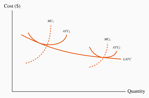
Consider the situation depicted in Figure 10.1. The
long-run ATC curve declines indefinitely. There is no output level where
average costs begin to increase. Imagine now having several firms, each
producing with a plant size corresponding to the short-run average cost
curve  , or alternatively a single larger firm using a plant size
denoted by
, or alternatively a single larger firm using a plant size
denoted by  . The small firms in this case cannot compete with the
larger firm because the larger firm has lower production costs and can
undercut the smaller firms, and supply the complete market in the
process. Such a scenario is termed a natural monopoly.
. The small firms in this case cannot compete with the
larger firm because the larger firm has lower production costs and can
undercut the smaller firms, and supply the complete market in the
process. Such a scenario is termed a natural monopoly.
Natural monopoly: one where the ATC of producing any output declines with the scale of operation.
Electricity distribution in some of Canada's provinces is in the hands of a
single supplier – Hydro Quebec or Hydro One in Ontario, for example. These distributors are natural monopolies in the sense described above: Unit distribution costs decline with size. In contrast, electricity production is not 'naturally' a monopoly. Other suppliers were once thought of as
'natural' monopolies also, but are no longer. Bell Canada was considered to be a natural monopoly in the era of land lines: It would not make economic sense to run several sets of phone lines to every residence. But that was before the arrival of cell phones, broadband and satellites. Canada Post was also thought to be a natural monopoly, until the advent of FEDEX, UPS and other couriers proved otherwise. Invention can compete away a 'natural' monopoly.
In reality there are very few pure monopolies. Facebook,
Microsoft, Amazon, Apple, Netflix and Google may be extraordinarily dominant in their
markets, but they are not the only suppliers of the services or products
that they offer. There exist other products that are similar.
National and Provincial Policy
Government policy can foster monopolies. Some governments are, or
once were, proud to have a 'national carrier' in the airline industry – Air
Canada in Canada or British Airways in the UK. The mail service was viewed
as a symbol of nationhood in Canada and the US: Canada Post and the
US Postal system are national emblems that have historic
significance. They were vehicles for integrating the provinces or states at
various points in the federal lives of these countries.
In the modern era, most of Canada's provinces have decided to create a
provincial monopoly crown corporation for the sale of cannabis. But
competition abounds in the form of an illegal market.
The down side of such nationalist policies is that they can be costly to the
taxpayer. Industries that are not subject to competition can become fat and
uncompetitive: Managers have insufficient incentives to curtail costs;
unions realize the government is committed to sustain the monopoly and push
for higher wages than under a more competitive structure, and innovation may be less likely to occur.
Maintaining barriers to entry
Monopolies can continue to survive if they
are successful in preventing the entry of new firms and products.
Patents and copyrights are one vehicle for preserving the sole-supplier
role, and are certainly necessary to encourage firms to undertake the
research and development (R&D) for new products.
Many corporations produce products that require a large up-front investment;
this might be in the form of research and development, or the construction
of costly production facilities. For example, Boeing or Airbus incurs billions of dollars in developing new aircraft;
pharmaceuticals may have to invest a billion dollars to develop a new drug.
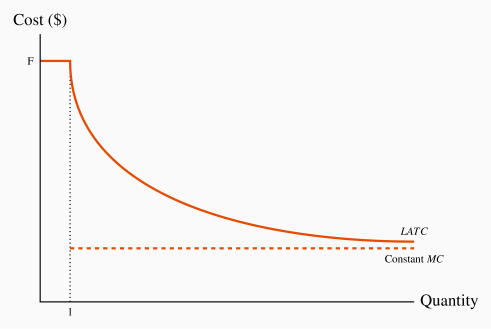
However, once such an investment is complete, the cost of producing each
unit of output may be relatively low. This is particularly true in pharmaceuticals. Such a phenomenon is displayed in Figure 10.2.
In this case the average cost for a small
number of units produced is high, but once the fixed cost is spread over an
ever larger output, the average cost declines rapidly, and in the limit
approaches the marginal cost. These production structures are common in
today's global economy, and they give rise to markets characterized either
by a single supplier or a small number of suppliers.
This figure is useful in understanding the role of patents. Suppose that
Pharma A spends one billion dollars in developing a new drug and
has constant unit production costs thereafter, while Pharma B
avoids research and development and simply imitates Pharma A's
product. Clearly Pharma B would have a LATC equal to its LMC,
and would be able to undercut the initial developer of the drug. Such an
outcome would discourage investment in new products and the economy at large
would suffer as a consequence. Economies would be worse off if protection is
not provided to the developers of new products because, if such protection
is not offered, potential developers will not have the incentive to incur the
up-front investment required.
While copyright and patent protection is legal, predatory pricing
is an illegal form of entry barrier, and we explore it more fully in Chapter 14. An example would be where an existing firm that sells
nationally may deliberately undercut the price of a small local entrant
to the industry. Airlines with a national scope are frequently accused of
posting low fares on flights in regional markets that a new carrier is
trying to enter.
Political lobbying is another means of maintaining monopolistic
power. For example, the Canadian Wheat Board had fought
successfully for decades to prevent independent farmers from marketing
wheat. This Board lost its monopoly status in August 2012, when the
government of the day decided it was not beneficial to consumers or farmers
in general. Numerous 'supply management' policies are in operation all
across Canada. Agriculture is protected by production quotas. All maple
syrup in Quebec must be marketed through a single monopoly supplier.
Critical networks also form a type of barrier, though not always a
monopoly. Microsoft's Office package has an almost monopoly status
in word processing and spreadsheet analysis for the reason that so many
individuals and corporations use it. The fact that we know a business
colleague will be able to edit our documents if written in Word,
provides us with an incentive to use Word, even if we might prefer
Wordperfect as a vehicle for composing documents. We develop the concept of strategic entry prevention further in Chapter 11.
10.2 Profit maximizing behaviour
We established in the previous chapter that, in deciding upon a
profit-maximizing output, any firm should produce up to the point where the
additional cost equals the additional revenue from a unit of output. What
distinguishes the supply decision for a monopolist from the supply decision
of the perfect competitor is that the monopolist faces a downward sloping
demand. A monopolist is the sole supplier and therefore must meet the full
market demand. This means that if more output is produced, the price must
fall. We will illustrate the choice of a profit maximizing output using
first a marginal-cost/marginal-revenue approach; then a supply/demand
approach.
Marginal revenue and marginal cost
Table 10.1 displays price and quantity values for
a demand curve in columns 1 and 2. Column 3 contains the sales revenue
generated at each output. It is the product of price and quantity. Since the
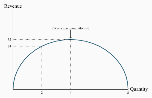
price denotes the revenue per unit, it is sometimes referred to as average revenue. The total revenue (TR) reaches a maximum at
$32, where 4 units of output are produced. A greater output necessitates a
lower price on every unit sold, and in this case revenue falls if the fifth
unit is brought to the market. Even though the fifth unit sells for a
positive price, the price on the other 4 units is now lower and the net
effect is to reduce total revenue. This pattern reflects what we examined in
Chapter 4: As price is lowered from the highest
possible value of $14 (where 1 unit is demanded) and the corresponding
quantity increases, revenue rises, peaks, and ultimately falls as output
increases. In Chapter 4 we explained that this maximum
revenue point occurs where the price elasticity is unity (-1), at the
midpoint of a linear demand curve.
Table 10.1 A profit maximizing monopolist
|
Quantity | Price | Total | Marginal | Marginal | Total | Profit |
|
(Q) | (P) | revenue (TR) | revenue (MR) | cost (MC) | cost (TC) | |
|
0 | 16 | | | | | |
|
1 | 14 | 14 | 14 | 2 | 2 | 12 |
|
2 | 12 | 24 | 10 | 3 | 5 | 19 |
|
3 | 10 | 30 | 6 | 4 | 9 | 21 |
|
4 | 8 | 32 | 2 | 5 | 14 | 18 |
|
5 | 6 | 30 | -2 | 6 | 20 | 10 |
|
6 | 4 | 24 | -6 | 7 | 27 | -3 |
|
7 | 2 | 14 | -10 | 8 | 35 | -21 |
Related to the total revenue function is the marginal revenue
function. It is the addition to total revenue due to the sale of one more
unit of the commodity.
Marginal revenue is the change in total revenue due to selling one more unit of the good.
Average revenue is the price per unit sold.
The MR in this example is defined in the fourth column of Table 10.1.
When the quantity sold increases from 1 unit to
2 units total revenue increases from $14 to $24. Therefore the marginal
revenue associated with the second unit of output is $10. When a third unit
is sold TR increases to $30 and therefore the MR of the third unit is
$6. As output increases the MR declines and eventually becomes negative
– at the point where the TR is a maximum: If TR begins to decline then
the additional revenue is by definition negative.
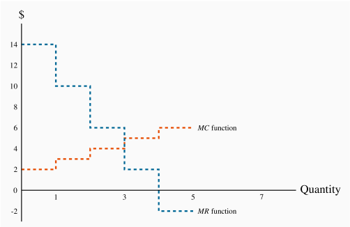
The MR function is plotted in Figure 10.4. It
becomes negative when output increases from 4 to 5 units.
The optimal output
This producer has a marginal cost structure given in the fifth column of the
table, and this too is plotted in Figure 10.4. Our
profit maximizing rule from Chapter 8 states that it is
optimal to produce a greater output as long as the additional revenue
exceeds the additional cost of production on the next unit of output. In
perfectly competitive markets the additional revenue is given by the fixed
price for the individual producer, whereas for the monopolist the additional
revenue is the marginal revenue. Consequently as long as MR exceeds MC
for the next unit a greater output is profitable, but once MC exceeds MR
the production of additional units should cease.
From Table 10.1 and Figure 10.4
it is clear that the optimal output is at 3 units.
The third unit itself yields a profit of 2$, the difference between MR
($6) and MC ($4). A fourth unit however would reduce profit by $3,
because the MR ($2) is less than the MC ($5). What price should the
producer charge? The price, as always, is given by the demand function. At a
quantity sold of 3 units, the corresponding price is $10, yielding total
revenue of $30.
Profit is the difference between total revenue and total cost. In Chapter 8
we computed total cost as the average cost times the
number of units produced. It can also be computed as the sum of costs
associated with each unit produced: The first unit costs $2, the second $3
and the third $4. The total cost of producing 3 units is the sum of these
dollar values: 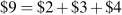 . The profit-maximizing output therefore
yields a profit of $21 (
. The profit-maximizing output therefore
yields a profit of $21 ( ).
).
Supply and demand
When illustrating market behaviour it is convenient to describe behaviour by
simple linear supply and demand functions that are continuous, rather than
the 'step' functions used in the preceding example. As explained in Chapter 5,
in using continuous curves to represent a market we
implicitly assume that a unit of output can be broken into subunits. In the
example above we assumed that sales always involve one whole unit of
the product being sold. In fact many goods can be sold in fractional units:
Gasoline can be sold in fractions of a litre; fruits and vegetables can be
sold in fractions of a kilogram, and so forth. Table 10.2 below furnishes
the data for our analysis.
Table 10.2 Discrete quantities
|
Price | Quantity | Total | Total | Profit |
|
| demanded | revenue | cost | |
|
12 | 0 | 0 | 0 | 0 |
|
11 | 2 | 22 | 1 | 21 |
|
10 | 4 | 40 | 4 | 36 |
|
9 | 6 | 54 | 9 | 45 |
|
8 | 8 | 64 | 16 | 48 |
|
7 | 10 | 70 | 25 | 45 |
|
6 | 12 | 72 | 36 | 36 |
|
5 | 14 | 70 | 49 | 21 |
|
4 | 16 | 64 | 64 | 0 |
|
3 | 18 | 54 | 81 | -27 |
|
2 | 20 | 40 | 100 | -60 |
|
1 | 22 | 22 | 121 | -99 |
|
0 | 24 | 0 | 144 | -144 |
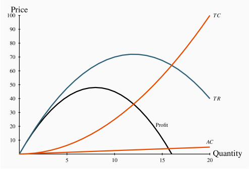
The first two columns define the demand curve. Total revenue is the product
of price and quantity and given in column 3. The cost data are given in
column 4, and profit – the difference between total revenue and total cost
is in the final column. Profit is maximized where the difference between
revenue and cost is greatest; in this case where the output is 8 units. At
lower or higher outputs profit is less. Figure 10.5 contains the curves
defining total revenue (TR), total cost (TC) and profit. These functions
can be obtained by mapping all of the revenue-quantity combinations, the
cost-quantity combinations, and the profit-quantity combinations as a series of
points, and joining these points to form the smooth functions displayed. The
vertical axis is measured in dollars, the horizontal axis in units of
output. Graphically, profit is maximized where the dollar difference between
TR and TC is greatest; that is at the output where the vertical distance
between the two curves is greatest. This difference, which is also defined
by the profit curve, occurs at a value of 8 units, corresponding to the
outcome in Table 10.2.
At any quantity less than this output, profit would rise with additional
output. This is because, from a less-than-optimal output, the additional
revenue from increased sales exceeds the increased cost associated with
producing those units: Stated differently, the marginal revenue would exceed
the marginal cost. Conversely, outputs greater than the optimum result in a
MR less than the associated MC. Accordingly, since outputs where MR>MC
are too low, and outputs where MR<MC are too high, the optimum must be
where the MR=MC. Hence, the equality between MR and MC is implied in
this diagram at the output where the difference between TR and TC is
greatest.
Note finally that total revenue is maximized where the TR curve reaches a
peak. In this example that occurs at a value of 12 units of output. This is
to be anticipated, as we learned in Chapter 4, because the midpoint of the
demand schedule in Table 10.2 occurs at that value.
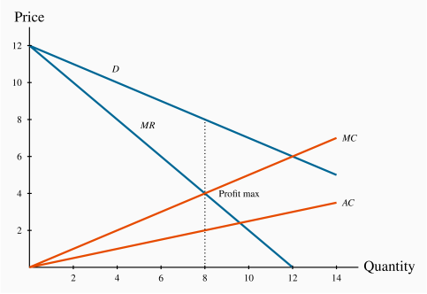
Figure 10.6 displays the demand curve for the market, the MR curve, and
the monopolist's MC and AC curves. Consider first the marginal revenue
curve. In contrast to the previous example, where only whole or integer
units could be sold, in this example units can be sold in fractional
amounts, and the MR curve must reflect this. To determine the position of
the MR curve, note that with a straight-line demand curve total revenue is
a maximum at the midpoint of the demand curve. Any increase in output
results in reduced revenue: Stated differently, the marginal revenue becomes
negative at that output. Up to that output the MR is positive, as
illustrated in Figure 10.3. Accordingly, the MR curve must intersect the
quantity axis midway between zero and the horizontal-axis intercept of the
demand curve. Geometrically, since the MR intersects the quantity axis
half way to the horizontal intercept of the demand curve, it must have a
slope that is twice the slope of the demand curve.
By observing the data in columns 1 and 2 of the table, the demand curve
intercepts are  , and from above discussion the MR curve
has intercepts
, and from above discussion the MR curve
has intercepts  . The AC is obtained by dividing TC by
output in Table 10.2, and the MC can be also
calculated as the change in total cost divided by the change in output
from Table 10.2. The result of these calculations
is displayed in Figure 10.6.
. The AC is obtained by dividing TC by
output in Table 10.2, and the MC can be also
calculated as the change in total cost divided by the change in output
from Table 10.2. The result of these calculations
is displayed in Figure 10.6.
The profit maximizing output is 8 units, where MC=MR. The price at which
8 units can be sold is read from the demand curve,
or the first column in Table 10.2. It is $8. And,
as expected, this price-quantity combination maximizes profit.
Table 10.2 indicates that profit is maximized at $48, at q=8.
Demand elasticity and marginal revenue
We have shown above that the MR curve cuts the horizontal axis at a
quantity where the elasticity of demand is unity. We know from Chapter 4
that demand is elastic at points on the demand curve
above this unit-elastic point. Furthermore, since the intersection of MR
and MC must be at a positive dollar value (MC cannot be negative), then
it must be the case that the profit maximizing price for a
monopolist always lies on the elastic segment of the demand curve.
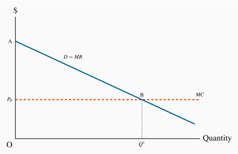
A general graphical representation
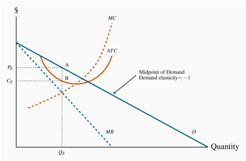
In Figure 10.7 we generalize the graphical representation of
the monopoly profit maximizing output by allowing the MC and ATC curves
to be nonlinear. The optimal output is at  , where MR=MC, and the
price
, where MR=MC, and the
price  sustains that output. With the average cost known, profit per
unit is AB, and therefore total profit is this margin multiplied by the
number of units sold, .
sustains that output. With the average cost known, profit per
unit is AB, and therefore total profit is this margin multiplied by the
number of units sold, .
Total profit is therefore 
Note that the monopolist may not always make a profit. Losses could result
in Figure 10.7 if average costs were to rise so that the ATC
were everywhere above the demand curve, or if the demand curve shifted down to
being everywhere below the ATC curve. In
the longer term the monopolist would have to either reduce costs or perhaps
stimulate demand through advertising if she wanted to continue in operation.
10.3 Long-run choices
Consider next the impact of a shift in demand upon the profit maximizing
choice of this firm. A rightward shift in demand in Figure 10.7
also yields a new MR curve. The firm therefore chooses a
new level of output, using the same profit maximizing rule: Set MC=MR.
This output will be greater than the previous output, but again the price
must be on an elastic portion of the new demand curve. If operating with the
same plant size, the MC and ATC curves do not change and the new profit
per unit is again read from the ATC curve.
By this stage the curious student will have asked: "What happens to plant
size in the long run?" For example, is the monopolist in Figure 10.7
using the most appropriate plant size in the first place?
Even if she is, should the monopolist consider adopting an expanded plant
size in response to the shift in demand?
The answer is: In the long run the monopolist is free to choose whatever
plant size is best. Her initial plant size might have been optimal for the
demand she faced, but if it was, it is unlikely to be optimal for the larger
scale of production associated with the demand shift. Accordingly, with the
new demand curve, she must consider how much profit she could make using
different plant sizes.
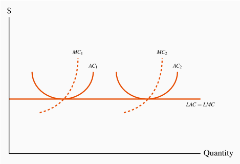
To illustrate one possibility, we will think of this firm as having constant
returns to scale at all output ranges, as displayed in Figure 10.8.
(Our reasoning carries through if the LAC slopes
downwards; the graph just becomes a little more complex.) The key
characteristic of constant returns to scale is that a doubling of inputs
leads to a doubling of output. Therefore, if the per-unit cost of inputs is
fixed, a doubling of inputs (and therefore output) leads exactly to a
doubling of costs. This implies that, when the firm varies its plant size
and its labour use, the cost of producing each additional unit must
be constant. The long-run marginal cost LMC is therefore constant and
equals the ATC in the long run.
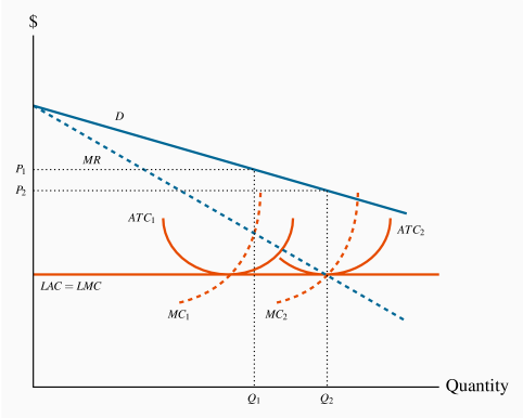
Figure 10.9 describes the market for this good. The optimal
output and price are determined in the usual manner: Set MC=MR. If the
monopolist has plant size corresponding to ATC1, the optimal output is
Q1 and should be sold at the price P1.The key issue now is: Given the
demand conditions, could the monopolist make more profit by choosing a plant
size that differs from the one corresponding to ATC1?
In this instance the answer is a clear 'yes'. Her LMC curve is horizontal
and so, by increasing output from Q1 to Q2 she earns a profit on each
additional unit in that range, because the MR curve lies above the LMC
curve. In order to produce the output level Q2 at least cost she must
choose a plant size corresponding to AC2.
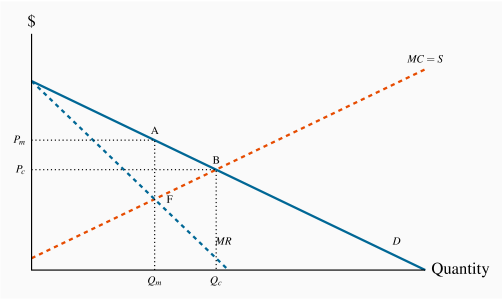
10.4 Output inefficiency
A characteristic of perfect competition is that it secures an efficient
allocation of resources when there are no externalities in the market:
Resources are used up to the point where their marginal cost equals their
marginal value – as measured by the price that consumers are willing to
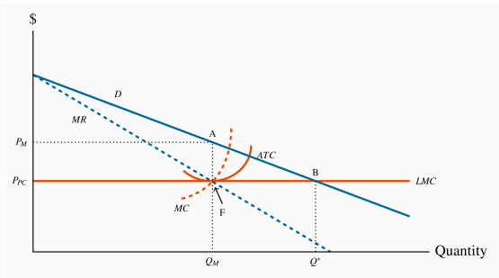
pay. But a monopoly structure does not yield this output. Consider Figure 10.10.
The monopolist's profit-maximizing output  is where MC equals MR.
This output is inefficient for the reason that we developed in Chapter 5:
If output is increased beyond the additional benefit
exceeds the additional cost of producing it. The additional benefit is
measured by the willingness of buyers to pay – the market demand curve. The
additional cost is the long-run MC curve under the assumption of constant
returns to scale. Using the terminology from Chapter 5,
there is a deadweight loss equal to the area ABF. This is termed
allocative inefficiency.
is where MC equals MR.
This output is inefficient for the reason that we developed in Chapter 5:
If output is increased beyond the additional benefit
exceeds the additional cost of producing it. The additional benefit is
measured by the willingness of buyers to pay – the market demand curve. The
additional cost is the long-run MC curve under the assumption of constant
returns to scale. Using the terminology from Chapter 5,
there is a deadweight loss equal to the area ABF. This is termed
allocative inefficiency.
Allocative inefficiency arises when resources are not appropriately allocated and result in deadweight losses .
Perfect competition versus monopoly
The area ABF can also be considered as the efficiency loss associated with
having a monopoly rather than a perfectly competitive market structure. In
perfect competition the supply curve is horizontal. This is achieved by
having firms enter and exit when more or less must be produced. Accordingly,
if the perfectly competitive industry's supply curve approximates
the monopolist's long-run marginal cost curve, we can say that if the monopoly were turned into a
competitive industry, output would increase from to  . The
deadweight loss is one measure of the superiority of the perfectly
competitive structure over the monopoly structure.
. The
deadweight loss is one measure of the superiority of the perfectly
competitive structure over the monopoly structure.
Note that this critique of monopoly is not initially focused upon profit.
While monopoly profits are what frequently irk the public, we have focused
upon resource allocation inefficiencies. But in a real sense the two are
related: Monopoly inefficiencies arise through output being restricted, and
it is this output reduction – achieved by maintaining a higher than
competitive price – that gives rise to those profits. Nonetheless, there is
more than just a shift in purchasing power from the buyer to the seller.
Deadweight losses arise because output is at a level lower than the point
where the MC equals the value placed on the good; thus the economy is
sacrificing the possibility of creating additional surplus.
Given that monopoly has this undesirable inefficiency, what measures should
be taken, if any, to counter the inefficiency? We will see what Canada's
Competition Act has to say in Chapter 14 and also examine
what other measures are available to control monopolies.
10.5 Price discrimination
A common characteristic in the pricing of many goods is that different
individuals pay different prices for goods or services that are essentially
the same. Examples abound: Seniors get a reduced rate for coffee in
Burger King; hair salons charge women more than they charge men; bank
charges are frequently waived for juniors. Price discrimination
involves charging different prices to different consumers in order to
increase profit.
Price discrimination involves charging different prices to different consumers in order to increase profit.
A strict definition of discrimination involves different prices for
identical products. We all know of a school friend who has been willing to
take the midnight flight to make it home at school break at a price he can
afford. In contrast, the business executive prefers the seven a.m.
flight to arrive for a nine a.m. business meeting in the same city
at several times the price. These are very mild forms of price
discrimination, since a midnight flight (or a midday flight) is not a
perfect substitute for an early morning flight. Price discrimination is
practiced because buyers are willing to pay different amounts for a good or
service, and the supplier may have a means of profiting from this. Consider
the following example.
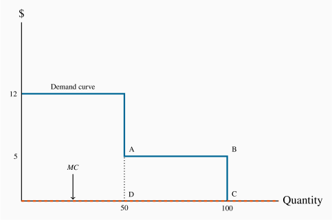
Family Flicks is the local movie theatre. It has two distinct
groups of customers – those of prime age form one group; youth and seniors
form the other. Family Flicks has done its market research and determined
that each group accounts for 50 percent of the total market of 100 potential
viewers per screening. It has also established that the prime-age group
members are willing to pay $12 to see a movie, while the seniors and youth
are willing to pay just $5. How should the tickets be priced?
Family Flicks has no variable costs, only fixed costs. It must pay a $100
royalty to the movie maker each time it shows the current movie, and must
pay a cashier and usher $20 each. Total costs are therefore $140,
regardless of how many people show up – short-run MC is zero. On the
pricing front, as illustrated in Table 10.3
below, if Family Flicks charges $12 per ticket it will attract 50 viewers,
generate $600 in revenue and therefore make a profit of $460.
Table 10.3 Price discrimination
|
| P=$5 | P=$12 | Twin price |
|
No. of customers | 100 | 50 | |
|
Total revenue | $500 | $600 | $850 |
|
Total costs | $140 | $140 | $140 |
|
Profit | $360 | $460 | $710 |
In contrast, if it charges $5 it can fill the theatre, because each of the
prime-age individuals is willing to pay more than $5, but the seniors and
youth are now offered a price they too are willing to pay. However, the
total revenue is now only $500 (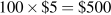 ), and profits are
reduced to $360. It therefore decides to charge the high price and leave
the theatre half-empty, because this strategy maximizes its profit.
), and profits are
reduced to $360. It therefore decides to charge the high price and leave
the theatre half-empty, because this strategy maximizes its profit.
Suppose finally that the theatre is able to segregate its customers. It can
ask the young and senior customers for identification upon entry, and in
this way charge them a lower price, while still maintaining the
higher price to the prime-age customers. If it can execute such a plan
Family Flicks can now generate $850 in revenue – $600 from the prime-age
group and $250 from the youth and seniors groups. Profit soars to $710.
There are two important conditions for this scheme to work:
The seller must be able to segregate the market at a
reasonable cost. In the movie case this is achieved by asking for
identification.
The second condition is that resale must be impossible or
impractical. For example, we rule out the opportunity for young buyers to
resell their tickets to the prime-age individuals. Sellers have many ways of
achieving this – they can require immediate entry to the movie theatre upon
ticket purchase, they can stamp the customer's hand, they can demand the
showing of ID with the ticket when entering the theatre area.
Frequently we think of sellers who offer price reductions to specific groups
as being generous. For example, hotels may levy only a nominal fee for the
presence of a child, once the parents have paid a suitable rate for the room
or suite in which a family stays. The hotel knows that if it charges too
much for the child, it may lose the whole family as a paying unit. The
coffee shop offering cheap coffee to seniors is interested in getting a
price that will cover its variable cost and so contribute to its profit. It
is unlikely to be motivated by philanthropy, or to be concerned with the
financial circumstances of seniors.
Price discrimination has a further interesting feature that is illustrated
in Figure 10.11: It frequently reduces the
deadweight loss associated with a monopoly seller!
In our Family Flicks example, the profit maximizing monopolist that did not,
or could not, price discriminate left 50 customers unsupplied who
were willing to pay $5 for a good that had a zero MC. This is a
deadweight loss of $250 because 50 seniors and youth valued a commodity at
$5 that had a zero MC. Their demand was not met because, in the absence
of an ability to discriminate between consumer groups, Family Flicks made
more profit by satisfying the demand of the prime-age group alone. But in this
example, by segregating its customers, the firm's profit maximization
behaviour resulted in the DWL being eliminated, because it supplied the
product to those additional 50 individuals. In this instance price
discrimination improves welfare, because more of a good is supplied in a
situation where market valuation exceeds marginal cost.
In the preceding example we simplified the demand side of the market by
assuming that every individual in a given group was willing to pay the same
price – either $12 or $5. More realistically each group can be defined by
a downward-sloping demand curve, reflecting the variety of prices that
buyers in a given market segment are willing to pay. It is valuable to
extend the analysis to include this reality. For example, a supplier may
face different demands from her domestic and foreign buyers, and if she can
segment these markets she can price discriminate effectively.
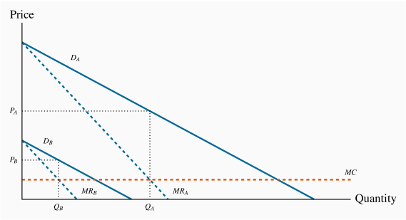
Consider Figure 10.12 where two segmented demands
are displayed, DA and DB, with their associated marginal revenue
curves, MRA and MRB. We will assume that marginal costs are constant
for the moment. It should be clear by this point that the profit maximizing
solution for the monopoly supplier is to supply an amount to each market
where the MC equals the MR in each market: Since the buyers in one
market cannot resell to buyers in the other, the monopolist considers these
as two different markets and therefore maximizes profit by applying the
standard rule. She will maximize profit in market A by supplying the
quantity QA and in market B by supplying QB. The prices at which these
quantities can be sold are PA and PB. These prices, unsurprisingly,
are different – the objective of segmenting markets is to increase profit
by treating the markets as distinct.
An example of this type of price discrimination is where pharmaceutical
companies sell drugs to less developed economies at a lower price than to
developed economies. The low price is sufficient to cover marginal cost and
is therefore profitable - provided the high price market covers the fixed
costs.
The preceding examples involved two separable groups of customers and are
very real. This kind of group segregation is sometimes called third
degree price discrimination. But it may be possible to segregate customers
into several groups rather than just two. In the limit, if we could charge a
different price to every consumer in a market, or for every unit sold, the
revenue accruing to the monopolist would be the area under the demand curve
up to the output sold. Though primarily of theoretical interest, this is
illustrated in Figure 10.13. It is termed perfect price discrimination, and sometimes first degree price
discrimination. Such discrimination is not so unrealistic: A tax accountant
may charge different customers a different price for providing the same
service; home renovators may try to charge as much as any client appears
willing to pay.
Second degree price discrimination is based on a different concept
of buyer identifiability. In the cases we have developed above, the seller
is able to distinguish the buyers by observing a vital
characteristic that signals their type. It is also possible that, while
individuals might have defining traits which influence their demands, such
traits might not be detectable by the supplier. Nonetheless, it is
frequently possible for the supplier to offer different pricing options
(corresponding to different uses of a product) that buyers would choose
from, with the result that her profit would be greater than under a uniform
price with no variation in the use of the service. Different cell phone
'plans', or different internet plans that users can choose from are examples
of this second-degree discrimination.
10.6 Cartels: Acting like a monopolist
A cartel is a group of suppliers that colludes to operate like
a monopolist. The cartel formed by the members of the Organization of Oil
Exporting Countries (OPEC) is an example of a cartel that was successful in
achieving its objectives for a long period. This cartel first flexed its
muscles in 1973, by increasing the world price of oil from $3 per barrel to
$10 per barrel. The result was to transfer billions of dollars from the
energy-importing nations in Europe and North America to OPEC members – the
demand for oil is relatively inelastic, hence an increase in price increases
total expenditures.
A cartel is a group of suppliers that colludes to operate like a monopolist.
A second renowned cartel is managed by De Beers, which controls a large part
of the world's diamond supply. In Canada, agricultural marketing boards are
a means of restricting supply legally. Such cartels may have thousands of
members. By limiting entry, through requiring a production 'quota', the
incumbents can charge a higher price than if entry to the industry were free.
To illustrate the dynamics of cartels consider Figure 10.14. Several producers, with given production capacities,
come together and agree to restrict output with a view to increasing price
and therefore profit. This may be done with the agreement of the government,
or it may be done secretively, and possibly against the law. Each firm has a
MC curve, and the industry supply is defined as the sum of these marginal
cost curves, as illustrated in Figure 9.3. The
resulting cartel is effectively one in which there is a single supplier with
many different plants – a multi-plant monopolist. To maximize profits this
organization will choose an output level  where the MR equals the MC. In contrast, if these firms act competitively the output chosen will be
 . The competitive output yields no supernormal profit, whereas the
monopoly/cartel output does.
. The competitive output yields no supernormal profit, whereas the
monopoly/cartel output does.
The cartel results in a deadweight loss equal to the area ABF, just as in
the standard monopoly model.
Cartel instability
Some cartels are unstable in the long run. In the first instance, the degree of instability depends on the authority
that the governing body of the cartel can exercise over its members, and
upon the degree of information it has on the operations of its members. If a
cartel is simply an arrangement among producers to limit output, each
individual member of the cartel has an incentive to increase its output,
because the monopoly price that the cartel attempts to sustain exceeds the
cost of producing a marginal unit of output. In Figure 10.14 each firm has a MC of output equal to $F when the
group collectively produces the output . Yet any firm that brings
output to market, beyond its agreed production limit, at the price  will make a profit of AF on that additional output – provided the other members of the cartel agree to restrict their output.
Since each firm faces the same incentive to increase output, it is difficult
to restrain all members from doing so.
will make a profit of AF on that additional output – provided the other members of the cartel agree to restrict their output.
Since each firm faces the same incentive to increase output, it is difficult
to restrain all members from doing so.
Individual members are more likely to abide by the cartel rules if the
organization can sanction them for breaking the supply-restriction
agreement. Alternatively, if the actions of individual members are not
observable by the organization, then the incentive to break ranks may be too
strong for the cartel to sustain its monopoly power.
We will see in Chapter 14 that Canada's Competition Act
forbids the formation of cartels, as it forbids many other anti-competitive
practices. At the same time, our governments frequently are the driving
force in the formation of domestic cartels.
In the second instance, cartels may be undermined eventually by the
emergence of new products and new technologies. OPEC has lost much of its
power in the modern era because of technological developments in oil
recovery. Canada's 'tar sands' yield oil, as a result of technological
developments that enabled producers to separate the oil from the earth it is
mixed with. Fracking technologies are another means of extracting oil
that is discovered in small pockets and encased in rock. The supply coming from these new technologies has limited the ability of the old OPEC cartel to increase prices through supply restriction.
Application Box 10.1 The taxi cartel
The new sharing economy has brought competition to some traditional cartels. City taxis are an example of such a formation: Traditionally, entry has been restricted to drivers who hold a permit (medallion), and fares are higher as a consequence of the resulting reduced supply. A secondary market then develops for these medallions, in which the city may offer new medallions through auction, or existing owners may exit and sell their medallions. Restricted entry has characterized most of Canada's major cities. Depending on the strictness of the entry process, medallions are worth correspondingly more. By 2012, medallions were selling in New York and Boston for a price in the neighborhood of one million dollars.
But ride-sharing start-up companies changed all of that. As Western examples, Uber and Lyft developed smart-phone apps that link demanders for rides with drivers, who may, or may not be, part of the traditional taxi companies. Such start-ups have succeeded in taking a significant part of the taxi business away from the traditional operators. As a result, the price of taxi medallions on the open market has plunged. From trading in the range of $1m. in New York in 2012, medallions are being offered in 2019 at about one fifth of that price. In Toronto, some medallions were traded in the range of $300,000 in 2012, but are on offer in 2019 for prices in the range of $30,000.
Not surprisingly, the traditional taxi companies charge that ride-hailing operators are violating the accepted rules governing the taxi business, and have launched legal suits against them and against local governments, and lobbied governments to keep them out of their cities.
In the new 'sharing economy', of which ride hailing companies are an example, participants operate with less traditional capital, and the communications revolution has been critical to their success. Home owners can use an online site to rent a spare bedroom in their house to visitors to their city (Airbnb), and thus compete with hotels. The main capital in this business is in the form of the information technology that links potential buyers to potential sellers.
Information on medallion prices in Canada can be found by, for example, searching at http://www.kijiji.ca
10.7 Invention, innovation and rent seeking
Invention and innovation are critical aspects of the modern economy. In
some sectors of the economy, firms that cannot invent or innovate are
liable to die. Invention is a genuine discovery, whereas innovation is
the introduction of a new product or process.
Invention is the discovery of a new product or process through research.
Product innovation refers to new or better goods or services.
Process innovation refers to new or better production or supply.
To this point we have said little that is good about monopolies. However,
the economist Joseph Schumpeter argued that, while monopoly leads to
resource misallocation in the economy, this cost might be offset by the
greater tendency for monopoly firms to invent and innovate. This is
because such firms have more profit and therefore more resources with
which to fund R&D and may therefore be more innovative than competitive
firms. If this were true then, taking a long-run dynamic view of the
marketplace, monopolies could have lower costs and more advanced products
than competitive firms and thus benefit the consumer.
While this argument has some logical appeal, it falls short on several
counts. First, even if large firms carry out more research than competitive
firms, there is no guarantee that the ensuing benefits carry over to the
consumer. Second, the results of such research may be used to prevent entry
into the industry in question. Firms may register their inventions and
gain use protection before a competitor can come up with the same or a
similar invention. Apple and Samsung each own tens of thousands of patents.
Third, the empirical evidence on the location of most R&D is inconclusive:
A sector with several large firms, rather than one with a single or very
many firms, may be best. For example, if Apple did not have Samsung as a
competitor, or vice versa, would the pace of innovation be as strong?
Fourth, much research has a 'public good' aspect to it. Research carried
out at universities and government-funded laboratories is sometimes
referred to as basic research: It explores the principles underlying
chemistry, social relations, engineering forces, microbiology, etc., and
has multiple applications in the commercial world. If disseminated, this
research is like a public good – its fruits can be used in many different
applications, and its use in one area does not preclude its use in others.
Consequently, rather than protecting monopolies on the promise of more R&D,
a superior government policy might be to invest directly in research and
make the fruits of the research publicly available.
Modern economies have patent laws, which grant inventors a
legal monopoly on use for a fixed period of time – perhaps fifteen years.
By preventing imitation, patent laws raise the incentive to conduct R&D
but do not establish a monopoly in the long run. Over the life of a patent
the inventor charges a higher price than would exist if his invention were
not protected; this both yields greater profits and provides the research
incentive. When the patent expires, competition from other producers leads
to higher output and lower prices for the product. Generic drugs are a good
example of this phenomenon.
Patent laws grant inventors a legal monopoly on use for a fixed period of time.
The power of globalization once again is very relevant in patents. Not all
countries have patent laws that are as strong as those in North America and
Europe. The BRIC economies (Brazil, Russia, India and China) form an emerging
power block. But their legal systems and enforcement systems are less
well-developed than in Europe or North America. The absence of a strong and
transparent legal structure inhibits research and development, because their
fruits may be appropriated by competitors.
Rent seeking
Citizens are frequently appalled when they read of lobbying activities in their
nation's capital. Every capital city in the world has an army of lobbyists,
seeking to influence legislators and regulators. Such individuals are in the
business of rent seeking, whose goal is to direct profit to
particular groups, and protect that profit from the forces of competition.
In Virginia and Kentucky we find that state taxes on cigarettes are
the lowest in the US – because the tobacco leaf is grown in these states,
and the tobacco industry makes major contributions to the campaigns of some
political representatives.
Rent-seeking carries a resource cost: Imagine that we could outlaw the lobbying
business and put these lobbyists to work producing goods and services in the
economy instead. Their purpose is to maintain as much quasi-monopoly
power in the hands of their clients as possible, and to ensure that the fruits
of this effort go to those same clients. If this practice could be curtailed then
the time and resources involved could be redirected to other productive ends.
Rent seeking is an activity that uses productive resources to redistribute rather than create output and value.
Industries in which rent seeking is most prevalent tend to be those in which
the potential for economic profits is greatest – monopolies or near-monopolies.
These, therefore, are the industries that allocate resources to the preservation
of their protected status. We do not observe laundromat owners or shoe-repair
businesses lobbying in Ottawa.
Conclusion
We have now examined two extreme types of market structure – perfect competition
and monopoly. While many sectors of the economy operate in a way that is close
to the competitive paradigm, very few are pure monopolies in that they have no close
substitute products. Even firms like Microsoft, or De Beers, that supply a huge
percentage of the world market for their product would deny that they are monopolies
and would argue that they are subject to strong competitive pressures from smaller
or 'fringe' producers. As a result we must look upon the monopoly paradigm as a useful
way of analyzing markets, rather than being an exact description of the world.
Accordingly, our next task is to examine how sectors with a few, several or multiple
suppliers act when pursuing the objective of profit maximization. Many different
market structures define the real economy, and we will concentrate on a limited
number of the more important structures in the next chapter.
Key Terms
Monopolist: is the sole supplier of an industry's output, and therefore the industry and the firm are one and the same.
Natural monopoly: one where the ATC of producing any output declines with the scale of operation.
Marginal revenue is the change in total revenue due to selling one more unit of the good.
Average revenue is the price per unit sold.
Allocative inefficiency arises when resources are not appropriately allocated and result in deadweight losses.
Price discrimination involves charging different prices to different consumers in order to increase profit.
A cartel is a group of suppliers that colludes to operate like a monopolist.
Rent seeking is an activity that uses productive resources to redistribute rather than create output and value.
Invention is the discovery of a new product or process through research.
Product innovation refers to new or better products or services.
Process innovation refers to new or better production or supply.
Patent laws grant inventors a legal monopoly on use for a fixed period of time.
Exercises for Chapter 10
Consider a monopolist with demand curve defined by P=100–2Q. The MR curve is MR=100–4Q and the marginal cost is MC=10+Q. The demand intercepts are  , the MR intercepts are
  .
.
Develop a diagram that illustrates this market, using either graph paper or an Excel spreadsheet, for values of output  .
.
Identify visually the profit-maximizing price and output combination.
Optional: Compute the profit maximizing price and output combination.
Consider a monopolist who wants to maximize revenue rather than profit. She has the demand curve P=72–Q, with marginal revenue MR=72–2Q, and MC=12. The demand intercepts are  , the MR intercepts are
  .
.
Graph the three functions, using either graph paper or an Excel spreadsheet.
Calculate the price she should charge in order to maximize revenue. [Hint: Where the MR=0.]
Compute the total revenue she will obtain using this strategy.
Suppose that the monopoly in Exercise 10.2 has a large number of plants. Consider what could happen if each of these plants became a separate firm, and acted competitively. In this perfectly competitive world you can assume that the MC curve of the monopolist becomes the industry supply curve.
Illustrate graphically the output that would be produced in the industry?
What price would be charged in the marketplace?
Optional: Compute the gain to the economy in dollar terms as a result of the DWL being eliminated [Hint: It resembles the area ABF in Figure 10.14].
In the text example in Table 10.1, compute the profit that the monopolist would make if he were able to price discriminate, by selling each unit at the demand price in the market.
A monopolist is able to discriminate perfectly among his consumers – by charging a different price to each one. The market demand curve facing him is given by P=72–Q. His marginal cost is given by MC=24 and marginal revenue is MR=72–2Q.
In a diagram, illustrate the profit-maximizing equilibrium, where discrimination is not practiced. The demand intercepts are , the MR intercepts are .
Illustrate the equilibrium output if he discriminates perfectly.
Optional: If he has no fixed cost beyond the marginal production cost of $24 per unit, calculate his profit in each pricing scenario.
A monopolist faces two distinct markets A and B for her product, and she is able to insure that resale is not possible. The demand curves in these markets are given by PA=20–(1/4)QA and PB=14–(1/4)QB. The marginal cost is constant: MC=4. There are no fixed costs.
Graph these two markets and illustrate the profit maximizing price and quantity in each market. [You will need to insert the MR curves to determine the optimal output.] The demand intercepts in A are  , and in B are
  .
.
In which market will the monopolist charge a higher price?
A concert organizer is preparing for the arrival of the Grateful Living band in his small town. He knows he has two types of concert goers: One group of 40 people, each willing to spend $60 on the concert, and another group of 70 people, each willing to spend $40. His total costs are purely fixed at $3,500.
Draw the market demand curve faced by this monopolist.
Draw the MR and MC curves.
With two-price discrimination what will be the monopolist's profit?
If he must charge a single price for all tickets can he make a profit?
Optional: A monopolist faces a demand curve P=64–2Q and MR=64–4Q. His marginal cost is MC=16.
Graph the three functions and compute the profit maximizing output and price.
Compute the efficient level of output (where MC=demand), and compute the DWL associated with producing the profit maximizing output rather than the efficient output.