10.3: Long-run choices

Last updated
Save as PDF

Page ID: 108411

\( \newcommand{\vecs}[1]{\overset { \scriptstyle \rightharpoonup} {\mathbf{#1}} } \) \( \newcommand{\vecd}[1]{\overset{-\!-\!\rightharpoonup}{\vphantom{a}\smash {#1}}} \)\(\newcommand{\id}{\mathrm{id}}\) \( \newcommand{\Span}{\mathrm{span}}\) \( \newcommand{\kernel}{\mathrm{null}\,}\) \( \newcommand{\range}{\mathrm{range}\,}\) \( \newcommand{\RealPart}{\mathrm{Re}}\) \( \newcommand{\ImaginaryPart}{\mathrm{Im}}\) \( \newcommand{\Argument}{\mathrm{Arg}}\) \( \newcommand{\norm}[1]{\| #1 \|}\) \( \newcommand{\inner}[2]{\langle #1, #2 \rangle}\) \( \newcommand{\Span}{\mathrm{span}}\) \(\newcommand{\id}{\mathrm{id}}\) \( \newcommand{\Span}{\mathrm{span}}\) \( \newcommand{\kernel}{\mathrm{null}\,}\) \( \newcommand{\range}{\mathrm{range}\,}\) \( \newcommand{\RealPart}{\mathrm{Re}}\) \( \newcommand{\ImaginaryPart}{\mathrm{Im}}\) \( \newcommand{\Argument}{\mathrm{Arg}}\) \( \newcommand{\norm}[1]{\| #1 \|}\) \( \newcommand{\inner}[2]{\langle #1, #2 \rangle}\) \( \newcommand{\Span}{\mathrm{span}}\)\(\newcommand{\AA}{\unicode[.8,0]{x212B}}\)

Consider next the impact of a shift in demand upon the profit maximizing choice of this firm. A rightward shift in demand in Figure 10.7 also yields a new MR curve. The firm therefore chooses a new level of output, using the same profit maximizing rule: Set MC=MR. This output will be greater than the previous output, but again the price must be on an elastic portion of the new demand curve. If operating with the same plant size, the MC and ATC curves do not change and the new profit per unit is again read from the ATC curve.

By this stage the curious student will have asked: "What happens to plant size in the long run?" For example, is the monopolist in Figure 10.7 using the most appropriate plant size in the first place? Even if she is, should the monopolist consider adopting an expanded plant size in response to the shift in demand?

The answer is: In the long run the monopolist is free to choose whatever plant size is best. Her initial plant size might have been optimal for the demand she faced, but if it was, it is unlikely to be optimal for the larger scale of production associated with the demand shift. Accordingly, with the new demand curve, she must consider how much profit she could make using different plant sizes.

Figure 10.8 The monopolist's choice of plant size

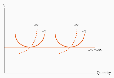
With constant returns to scale and constant prices per unit of labour and capital, a doubling of output involves exactly a doubling of costs. Thus, per unit costs, or average costs, are constant in the LR. Hence LAC=LMC, and each is constant.

To illustrate one possibility, we will think of this firm as having constant returns to scale at all output ranges, as displayed in Figure 10.8. (Our reasoning carries through if the LAC slopes downwards; the graph just becomes a little more complex.) The key characteristic of constant returns to scale is that a doubling of inputs leads to a doubling of output. Therefore, if the per-unit cost of inputs is fixed, a doubling of inputs (and therefore output) leads exactly to a doubling of costs. This implies that, when the firm varies its plant size and its labour use, the cost of producing each additional unit must be constant. The long-run marginal cost LMC is therefore constant and equals the ATC in the long run.

Figure 10.9 describes the market for this good. The optimal output and price are determined in the usual manner: Set MC=MR. If the monopolist has plant size corresponding to ATC₁, the optimal output is Q₁ and should be sold at the price P₁.The key issue now is: Given the demand conditions, could the monopolist make more profit by choosing a plant size that differs from the one corresponding to ATC₁?

Figure 10.9 Plant size in the long run

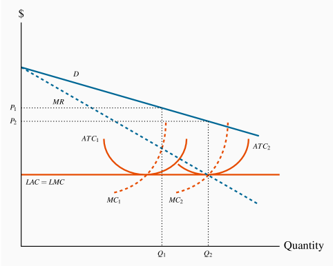
With demand conditions defined by D and MR, the optimal plant size is one corresponding to the point where MR=MC in the long run. Therefore Q₂ is the optimal output and the optimal plant size corresponds to ATC₂. If the current plant is defined by ATC₁, then optimal SR production is Q₁.

In this instance the answer is a clear 'yes'. Her LMC curve is horizontal and so, by increasing output from Q₁ to Q₂ she earns a profit on each additional unit in that range, because the MR curve lies above the LMC curve. In order to produce the output level Q₂ at least cost she must choose a plant size corresponding to AC₂.