In this chapter we will explore:
| 13.1 | The concept of human capital
|
| 13.2 | Productivity and education
|
| 13.3 | On-the-job training
|
| 13.4 | Education as signaling
|
| 13.5 | Returns to education and education quality
|
| 13.6 | Discrimination
|
| 13.7 | The income and earnings distribution in Canada
|
| 13.8 | Wealth and capitalism
|
Individuals with different characteristics earn different amounts because
their productivity levels differ. While it is convenient to work with a
single marginal productivity of labour function to illustrate the
functioning of the labour market, as we did in Chapter 12,
for the most part wages and earnings vary by
education level and experience, and sometimes by ethnicity and gender. In
this chapter we develop an understanding of the sources of these
differentials, and how they are reflected in the distribution of income.
13.1 Human capital
Human capital, HK, is the stock of knowledge and ability
accumulated by a worker that determines future productivity and earnings. It
depends on many different attributes – education, experience, intelligence,
interpersonal skills etc. While human capital influences own earnings, it also impacts the productivity of the
economy at large, and is therefore a vital force in determining long-run
growth. Canada has been investing heavily in human
capital in recent decades, and this suggests that future productivity and
earnings will benefit accordingly.
Human capital is the stock of knowledge and ability accumulated by a worker that determines future productivity and earning.
Several features of Canada's recent human capital accumulation are
noteworthy. First, Canada's enrollment rate in post-secondary education now
exceeds the US rate, and that of virtually every economy in the world.
Second is the fact that the number of women in third-level institutions
exceeds the number of men. Almost 60% of university students are women.
Third, international testing of high-school students sees Canadian students
performing well, which indicates that the quality of the Canadian
educational system appears to be high. These are positive aspects of a
system that frequently comes under criticism. Nonetheless, the distribution
of income that emerges from market forces in Canada has become more unequal.
Let us now try to understand individuals' economic motivation for embarking on the
accumulation of human capital, and in the process see why different groups
earn different amounts. We start by analyzing the role of education and then
turn to on-the-job training. At the outset, we
recognize that many individuals acquire knowledge for its own sake or in
order to improve the quality of their lives. Education can improve one's
appreciation of art, literature and the sciences.
13.2 Productivity and education
Human capital is the result of past investment that raises future incomes. A
critical choice for individuals is to decide upon exactly how much
additional human capital to accumulate. The cost of investing in another
year of school is the direct cost, such as school fees, plus the
indirect, or opportunity, cost, which can be measured by the
foregone earnings during that extra year. The benefit of the additional
investment is that the future flow of earnings is augmented. Consequently,
wage differentials should reflect different degrees of education-dependent
productivity.
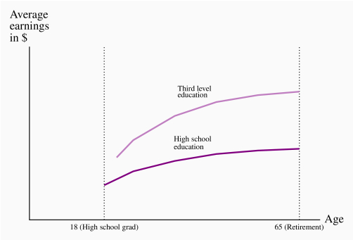
Age-earnings profiles
Figure 13.1 illustrates two typical age-earnings profiles for individuals with different levels of
education. These profiles define the typical pattern of earnings over time,
and are usually derived by examining averages across individuals in surveys.
Two aspects are clear: People with more education not only earn more, but
the spread tends to grow with time. Less educated, healthy young individuals
who work hard may earn a living wage but, unlike their more educated
counterparts, they cannot look forward to a wage that rises substantially
over time. More highly-educated individuals go into jobs and occupations
that take a longer time to master: Lawyers, doctors and most professionals
not only undertake more schooling than truck drivers, they also spend many
years learning on the job, building up a clientele and accumulating
expertise.
Age-earnings profiles define the pattern of earnings over time for individuals with different characteristics.
The education premium
Individuals with different education levels earn different wages. The education premium is the difference in earnings between the
more and less highly educated. Quantitatively, Professors Kelly Foley and
David Green have recently proposed that the completion of a college or trade
certification adds about 15% to one's income, relative to an individual who
has completed high school. A Bachelor's degree brings a premium of 20-25%,
and a graduate degree several percentage points more. The failure to
complete high school penalizes individuals to the extent of about 10%.
These are average numbers, and they vary depending upon the province of
residence, time period and gender. Nonetheless the findings underline that
more human capital is associated with higher earnings. The earnings premium
depends upon both the supply and demand of high HK individuals.
Ceteris paribus, if high-skill workers are heavily in demand by employers,
then the premium should be greater than if lower-skill workers are more in
demand.
Education premium: the difference in earnings between the more and less highly educated.
The distribution of earnings has become more unequal in Canada and the US in
recent decades, and one reason that has been proposed for this development
is that the modern economy demands more high-skill workers; in particular
that technological change has a bigger impact on productivity when combined
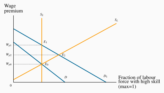
with high-skill workers than with low-skill workers. Consider Figure 13.2
which contains supply and demand functions with a
twist. We imagine that there are two types of labour: One with a high level
of human capital, the other with a lower level. The vertical axis measures
the wage premium of the high-education group (which can be measured
in dollars or percentage terms), and the horizontal axis measures the
fraction of the total labour force that is of the high-skill type.
D is the relative demand for the high skill workers, in this
example for the economy as a whole. There is some degree of substitution
between high and low-skill workers in the modern economy. We do not propose
that several low-skill workers can perform the work of one neuro-surgeon;
but several individual households (low-skill) could complete their income tax
submissions in the same time as one skilled tax specialist. In this example
there is a degree of substitutability. In a production environment, a
high-skill manager, equipped with technology and capital, can perform the
tasks of several line workers.
The demand curve D defines the premium that employers (demanders) are willing to pay
to the higher skill group. The negative slope indicates that if demanders
were to employ a high proportion of skilled workers, the premium they would
be willing to pay would be less than if they demanded a smaller share of
high-skilled workers, and a larger share of lower-skilled workers. The wage
premium for high HK individuals at any given time is determined by the
intersection of supply and demand.
In the short run the make-up of the labour force is fixed, and this is
reflected in the vertical supply curve Ss. The equilibrium is at E0,
and  is the premium, or excess, paid to the higher-skill worker over
the lower-skill worker. In the long run it is possible for the economy to
change the composition of its labour supply: If the wage premium increases,
more individuals will find it profitable to train as high-skill workers.
That is to say, the fraction of the total that is high-skill increases. It
follows that the long-run supply curve slopes upwards.
is the premium, or excess, paid to the higher-skill worker over
the lower-skill worker. In the long run it is possible for the economy to
change the composition of its labour supply: If the wage premium increases,
more individuals will find it profitable to train as high-skill workers.
That is to say, the fraction of the total that is high-skill increases. It
follows that the long-run supply curve slopes upwards.
So what happens when there is an increase in the demand for high-skill
workers relative to low-skill workers? The demand curve shifts upward to
 , and the new equilibrium is at
  . The supply mix is fixed in
the short run, so there is an increase in the wage premium. But over time,
some individuals who might have been just indifferent between educating
themselves more and going into the workplace with lower skill levels now
find it worthwhile to pursue further education. Their higher anticipated
returns to the additional human capital they invest in now exceed the
additional costs of more schooling, whereas before the premium increase
these additional costs and benefits were in balance. In Figure 13.2
the new short-run equilibrium at has a
corresponding wage premium of
. The supply mix is fixed in
the short run, so there is an increase in the wage premium. But over time,
some individuals who might have been just indifferent between educating
themselves more and going into the workplace with lower skill levels now
find it worthwhile to pursue further education. Their higher anticipated
returns to the additional human capital they invest in now exceed the
additional costs of more schooling, whereas before the premium increase
these additional costs and benefits were in balance. In Figure 13.2
the new short-run equilibrium at has a
corresponding wage premium of  . In the long run, after additional
supply has reached the market, the increased premium is moderated to
. In the long run, after additional
supply has reached the market, the increased premium is moderated to  at the equilibrium
  .
.
This figure displays what many economists believe has happened in North
America in recent decades: The demand for high HK individuals has increased,
and the additional supply has not been as great. Consequently the wage
premium for the high-skill workers has increased. As we describe later in
this chapter, that is not the only perspective on what has happened.
Are students credit-constrained or culture-constrained?
The foregoing analysis assumes that students and potential students make
rational decisions on the costs and benefits of further education and act
accordingly. It also assumes implicitly that individuals can borrow the
funds necessary to build their human capital: If the additional returns to
further education are worthwhile, individuals should borrow the money to
make the investment, just as entrepreneurs do with physical capital.
However, there is a key difference in the credit markets. If an entrepreneur
fails in her business venture the lender will have a claim on the physical
capital. But a bank cannot repossess a human being who drops out of school
without having accumulated the intended human capital. Accordingly, the
traditional lending institutions are frequently reluctant to lend the amount
that students might like to borrow—students are credit constrained. The
sons and daughters of affluent families therefore find it easier to attend
university, because they are more likely to have a supply of funds
domestically. Governments customarily step into the breach and supply loans
and bursaries to students who have limited resources. While funding
frequently presents an obstacle to attending a third-level institution, a
stronger determinant of attendance is the education of the parents, as
detailed in Application Box 13.1.
Application Box 13.1 Parental education and university attendance in Canada
The biggest single determinant of university attendance in the modern era is parental education. A recent study* of who goes to university examined the level of parental education of young people 'in transition' – at the end of their high school – for the years 1991 and 2000.
For the year 2000 they found that, if a parent had not completed high school, there was just a 12% chance that their son would attend university and an 18% chance that a daughter would attend. In contrast, for parents who themselves had completed a university degree, the probability that a son would also attend university was 53% and for a daughter 62%. Hence, the probability of a child attending university was roughly four times higher if the parent came from the top educational category rather than the bottom category! Furthermore the authors found that this probability gap opened wider between 1991 and 2000.
In the United States, Professor Sear Reardon of Stanford University has followed the performance of children from low-income households and compared their achievement with children from high-income households. He has found that the achievement gap between these groups of children has increased substantially over the last three decades. The reason for this growing separation is not because children from low-income households are performing worse in school, it is because high-income parents invest much more of their time and resources in educating their children, both formally in the school environment, and also in extra-school activities.
*Finnie, R., C. Laporte and E. Lascelles. "Family Background and Access to Post-Secondary Education: What Happened in the Nineties?" Statistics Canada Research Paper, Catalogue number 11F0019MIE-226, 2004
Reardon, Sean, "The Great Divide", New York Times, April 8, 2015.
13.3 On-the-job training
As is clear from Figure 13.1, earnings are
raised both by education and experience. Learning on the job is central to
the age-earnings profiles of the better educated, and is less important for
those with lower levels of education. On-the-job training
improves human capital through work experience. If on-the-job training
increases worker productivity, who should pay for this learning – firms or
workers? To understand who should pay, we distinguish between two kinds of
skills: Firm-specific skills that raise a worker's
productivity in a particular firm, and general skills that
enhance productivity in many jobs or firms.
Firm-specific HK could involve knowing how particular components of a
somewhat unique production structure functions, whereas general human
capital might involve an understanding of engineering or architectural
principles that can be applied universally. As for who should pay for the
accumulation of skills: An employer should be willing to undertake most of
the cost of firm-specific skills, because they are of less value to the
worker should she go elsewhere. Firms offering general or transferable
training try to pass the cost on to the workers, perhaps by offering a
wage-earnings profile that starts very low, but that rises over time.
Low-wage apprenticeships are examples. Hence, whether an employee is a
medical doctor in residence, a plumber in an apprenticeship or a young
lawyer in a law partnership, she 'pays' for the accumulation of her portable
HK by facing a low wage when young. Workers are willing to accept such an
earnings profile because their projected future earnings will compensate for
lower initial earning.
On-the-job training improves human capital through work experience.
Firm-specific skills raise a worker's productivity in a particular firm.
General skills enhance productivity in many jobs or firms.
13.4 Education as signalling
An alternative view of education springs from the theory of signalling. This
is a provocative theory that proposes education may be worthwhile, even if
it generates little additional skills. The theory recognizes that
individuals possess different abilities. However, firms cannot easily
recognize the more productive workers without actually hiring them and
finding out ex-post – sometimes a costly process. Signalling theory says that, in pursuing more education,
people who know they are more capable thereby send a signal to potential employers
that they are the more capable workers. Education therefore screens out the low-productivity workers from the
high-productivity (more educated) workers. Firms pay more to the latter,
because firms know that the high-ability workers are those with the
additional education.
Signalling is the decision to undertake an action in order to reveal information.
Screening is the process of obtaining information by observing differences in behaviour.
To be effective, the process must separate the two types. Why don't
lower-ability workers go to university and pretend they are of the
high-ability type? Primarily because that strategy could backfire: Such
individuals are less likely to succeed at school and there are costs
associated with school in the form of school fees, books and foregone
earnings. While they may have lower innate skills, they are likely smart
enough to recognize a bad bet.
On balance economists believe that further education does indeed add to
productivity, although there may be an element of screening present: An
engineering degree (we should hope) increases an individual's understanding
of mechanical forces so that she can design a bridge that will not collapse,
in addition to telling a potential employer that the student is smart!
Finally, it should be evident that if education raises productivity, it is
also good for society and the economy at large.
13.5 Education returns and quality
How can we be sure that further education really does generate the returns,
in the form of higher future incomes, to justify the investment? For many
years econometricians proposed that an extra year of schooling might offer a
return in the region of 10% – quite a favourable return in comparison with
what is frequently earned on physical capital. Doubters then asked if the
econometric estimation might be subject to bias – what if the additional
earnings of those with more education are simply attributable to the fact
that it is the innately more capable individuals who both earn more and who
have more schooling? And since we cannot observe who has more innate
ability, how can we be sure that it is the education itself, rather than
just differences in ability, that generate the extra income?
This is a classical problem in inference: Does correlation imply causation?
The short answer to this question is that education economists are convinced
that the time invested in additional schooling does indeed produce
additional rewards, even if it is equally true that individuals who are
innately smarter do choose to invest in that way. Furthermore, it appears
that the returns to graduate education are higher than the returns to
undergraduate education.
What can be said of the quality of different educational systems? Are
educational institutions in different countries equally good at producing
knowledgeable students? Or, viewed another way: Has a grade nine student in
Canada the same skill set as a grade nine student in France or Hong Kong? An
answer to this question is presented in Table 13.1,
which contains results from the Program for International Student Assessment
(PISA) – an international survey of 15-year old student abilities in
mathematics, science and literacy. This particular table presents the
results for a sample of the countries that were surveyed. The results
indicate that Canadian students perform well in all three dimensions of the
test.
Table 13.1 Mean scores in PISA tests
|
Country | Math | Science | Reading |
|
Australia | 494 | 510 | 503 |
|
Austria | 497 | 495 | 485 |
|
Belgium | 507 | 502 | 499 |
|
Canada | 516 | 528 | 527 |
|
Denmark | 511 | 502 | 500 |
|
Finland | 511 | 531 | 526 |
|
France | 493 | 495 | 499 |
|
Germany | 506 | 509 | 509 |
|
Greece | 454 | 455 | 467 |
|
Hong Kong | 548 | 523 | 527 |
|
Ireland | 504 | 503 | 521 |
|
Italy | 490 | 481 | 485 |
|
Japan | 532 | 538 | 516 |
|
Korea | 524 | 516 | 517 |
|
Mexico | 408 | 416 | 423 |
|
New Zealand | 495 | 513 | 509 |
|
Norway | 502 | 498 | 513 |
|
Spain | 486 | 493 | 496 |
|
Sweden | 494 | 493 | 500 |
|
Switzerland | 521 | 506 | 492 |
|
Turkey | 420 | 425 | 428 |
|
United States | 470 | 496 | 497 |
|
United Kingdom | 492 | 509 | 498 |
An interesting paradox arises at this point: If productivity growth in
Canada has lagged behind some other economies in recent decades, as many
economists believe, how can this be explained if Canada produces
many well-educated high-skill workers? The answer may
be that there is a considerable time lag before high participation rates in
third-level education and high quality make themselves felt on the national
stage in the form of elevated productivity. The evidence suggests a good
productivity future, in so far as it depends upon human capital. At the same time, if
investment in human capital is not matched by investment in physical capital
then the human capital may not be able to perform to its ability.
13.6 Discrimination
Wage differences are a natural response to differences in human capital. But
we frequently observe wage differences that might be discriminatory. For
example, women on average earn less than men with similar qualifications;
older workers may be paid less than those in their prime years; immigrants
may be paid less than native-born Canadians, and ethnic minorities may be
paid less than traditional white workers. The term discrimination describes an earnings differential that is
attributable to a trait other than human capital.
If two individuals have the same HK, in the broadest sense of having the
same capability to perform a particular task, then a wage premium paid to
one represents discrimination. Correctly measured then, the discrimination
premium between individuals from these various groups is the differential in
earnings after correcting for HK differences. Thousands of studies have been
undertaken on discrimination, and most conclude that discrimination abounds.
Women, particularly those who have children, are paid less than men, and
frequently face a 'glass ceiling' – a limit on their promotion
possibilities within organizations.
Discrimination implies an earnings differential that is attributable to a trait other than human capital.
In contrast, women no longer face discrimination in university and college
admissions, and form a much higher percentage of the student population than
men in many of the higher paying professions such as medicine and law.
Immigrants to Canada also suffer from a wage deficit. This is especially
true for the most recent cohorts of working migrants who now come
predominantly, not from Europe, as was once the case, but from China, South
Asia, Africa and the Caribbean. For similarly-measured HK as Canadian-born
individuals, these migrants frequently have an initial wage deficit of 30%,
and require a period of more than twenty years to catch-up. How much of this
differential might be due to the quality of the education or human capital
received abroad is difficult to determine.
13.7 The income distribution
How does all of our preceding discussion play out when it comes to the
income distribution? That is, when we examine the incomes of all individuals
or households in the economy, how equally or unequally are they distributed?
The study of inequality is a critical part of economic analysis. It
recognizes that income differences that are in some sense 'too large' are
not good for society. Inordinately large differences can reflect poverty and
foster social exclusion and crime. Economic growth that is concentrated in
the hands of the few can increase social tensions, and these can have
economic as well as social or psychological costs. Crime is one reflection
of the divide between 'haves' and 'have-nots'. It is economically costly;
but so too is child poverty. Impoverished children rarely achieve their
social or economic potential and this is a loss both to the individual and society at large.
In this section we will first describe a subset of the basic statistical
tools that economists use to measure inequality. Second, we will examine how
income inequality has evolved in recent decades. We shall see that, while
the picture is complex, market income inequality has indeed increased in
Canada. Third, we shall investigate some of the proposed reasons for the
observed increase in inequality. Finally we will examine if the government
offsets the inequality that arises from the marketplace through its taxation
and redistribution policies.
It is to be emphasized that income inequality is just one proximate measure
of the distribution of wellbeing. The extent of poverty is another such
measure. Income is not synonymous with happiness but, that being said,
income inequality can be computed reliably, and it provides a good measure
of households' control over economic resources.
Theory and measurement
Let us rank the market incomes of
all households in the economy from poor to rich, and categorize this
ordering into different quantiles or groups. With five such quantiles the
shares are called quintiles. The richest group forms the highest
quintile, while the poorest group forms the lowest quintile. Such a
representation is given in Table 13.2. The first
numerical column displays the income in each quintile as a percentage of
total income. If we wanted a finer breakdown, we could opt for decile (ten),
or even vintile (twenty) shares, rather than quintile shares. These data can
be graphed in a variety of ways. Since the data are in share, or percentage,
form, we can compare, in a meaningful manner, distributions from economies
that have different average income levels.
Table 13.2 Quintile shares of total family income in Canada, 2011
|
| Quintile share of total income | Cumulative share |
|
First quintile | 4.1 | 4.1 |
|
Second quintile | 9.6 | 13.7 |
|
Third quintile | 15.3 | 29.0 |
|
Fourth quintile | 23.8 | 52.8 |
|
Fifth quintile | 47.2 | 100.0 |
|
Total | 100 | |
Source: Statistics Canada, CANSIM Matrix 2020405. These combinations are represented by the circles in the figure.
An informative way of presenting these data graphically is to plot the
cumulative share of income against the cumulative share of the population.
This is given in the final column, and also presented graphically in Figure 13.3. The bottom quintile has 4.1% of total income.
The bottom two quintiles together have  , and so forth.
By joining the coordinate pairs represented by the circles, a Lorenz curve is obtained. Relative to the diagonal line it is
a measure of how unequally incomes are distributed: If everyone had the same
income, each 20% of the population would have 20% of total income and by
joining the points for such a distribution we would get a straight diagonal
line joining the corners of the box. In consequence, if the Lorenz curve is
further from the line of equality the distribution is less equal than if the
Lorenz curve is close to the line of equality.
, and so forth.
By joining the coordinate pairs represented by the circles, a Lorenz curve is obtained. Relative to the diagonal line it is
a measure of how unequally incomes are distributed: If everyone had the same
income, each 20% of the population would have 20% of total income and by
joining the points for such a distribution we would get a straight diagonal
line joining the corners of the box. In consequence, if the Lorenz curve is
further from the line of equality the distribution is less equal than if the
Lorenz curve is close to the line of equality.
Lorenz curve describes the cumulative percentage of the income distribution going to different quantiles of the population.
This suggests that the area A relative to the area (A + B) forms a measure
of inequality in the income distribution. This fraction obviously lies
between zero and one, and it is called the Gini index. A
larger value of the Gini index indicates that inequality is greater. We will
not delve into the mathematical formula underlying the Gini, but for this
set of numbers its value is 0.4.
Gini index: a measure of how far the Lorenz curve lies from the line of equality. Its maximum value is one; its minimum value is zero.
The Gini index is what is termed summary index of inequality – it
encompasses a lot of information in one number. There exist very many other
such summary statistics.
It is important to recognize that very different Gini index values emerge
for a given economy by using different income definitions of the variable
going into the calculations. For example, the quintile shares of the
earnings of individuals rather than the incomes of households
could be very different. Similarly, the shares of income post tax
and post transfers will differ from their shares on a pre-tax,
pre-transfer basis.
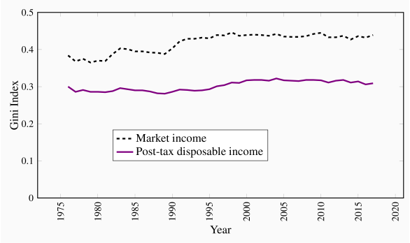
Figure 13.4 contains Gini index values for two
different definitions of income from 1976 to 2011. The upper line
represents the Gini index values for households where the income measure is
market income; the lower line defines the Gini values when income is defined
as post-tax and post-transfer incomes. The latter income measure deducts
taxes paid and adds income such as Employment Insurance or Social Assistance
benefits. Two messages emerge from this graphic: The first is that the
distribution of market incomes displays more inequality than the
distribution of incomes after the government has intervened. In the latter
case incomes are more equally distributed than in the former. The second
message to emerge is that inequality increased over time – the Gini
values are larger in the years after approximately 2000 than in the earlier years, although the
increase in market income inequality is greater than the increase in income
inequality based on a 'post-government' measure of income.
This is a very brief description of recent events. It is also possible to
analyze inequality among women and men, for example, as well as among
individuals and households. But the essential message remains clear:
Definitions are important; in particular the distinction between incomes
generated in the market place and incomes after the government has
intervened through its tax and transfer policies.
Application Box 13.2 The very rich
McMaster University Professor Michael Veall and his colleague Emmanuel Saez, from University of California, Berkeley, have examined the evolution of the top end of the Canadian earnings distribution in the twentieth century. Using individual earnings from a database built upon tax returns, they show how the share of the very top of the distribution declined in the nineteen thirties and forties, remained fairly stable in the decades following World War II, and then increased from the eighties to the present time. The increase in share is particularly strong for the top 1% and even stronger for the top one tenth of the top 1%. These changes are driven primarily by changes in earnings, not on stock options awarded to high-level corporate employees. The authors conclude that the change in this region of the distribution is attributable to changes in social norms. Whereas, in the nineteen eighties, it was expected that a top executive would earn perhaps a half million dollars, the 'norm' has become several million dollars in the present day. Such high remuneration became a focal point of public discussion after so many banks in the United States in 2008 and 2009 required government loans and support in order to avoid collapse. It also motivated the many 'occupy' movements of 2011 and 2012, and the US presidential race in 2019.
Saez, E. and M. Veall. "The evolution of high incomes in Canada, 1920-2000." Department of Economics research paper, McMaster University, March 2003.
In the international context, Canada is neither a strongly egalitarian
economy nor one characterized by great income inequality. OECD data indicate
that the economies with the lowest Gini index values are the Czech and
Slovak republics and Iceland, with values in the neighborhood of 0.25 based
on a post-government measure of income. Canada has a Gini index of .31, the
US a value of .38 and at the upper end are economies such as Mexico and
Chile with values of .47 (https://data.oecd.org/inequality/income-inequality.htm).
Economic forces
The increase in inequality of earnings in the market place in Canada has
been reflected in many other developed economies – to a greater degree in
the US and to a lesser extent in some European economies. Economists have
devoted much energy to studying why, and as a result there are several
accepted reasons.
Younger workers and those with lower skill levels have faired poorly in the
last three decades. Globalization and out-sourcing
have put pressure on low-end wages. In effect the workers in the lower tail of
the distribution are increasingly competing with workers from low-wage
less-developed economies. While this is a plausible causation, the critics
of the perspective point out that wages at the bottom have fallen not only
for those workers who compete with overseas workers in manufacturing, but
also in the domestic services sector right across the economy. Obviously the
workers at McDonalds have not the same competition from low-wage economies
as workers who assemble toys.
A competing perspective is that it is technological change that has enabled
some workers to do better than others. In explaining why high wage workers
in many economies have seen their wages increase, whereas low-wage workers
have seen a relative decline, the technological change hypothesis proposes
that the form of recent technological change is critical: Change has been
such as to require other complementary skills and education in order to
benefit from it. For example, the introduction of computer-aided design
technology is a benefit to workers who are already skilled and earning a
high wage: Existing high skills and technological change are
complementary. Such technological change is therefore different from the
type underlying the production line. Automation in the early twentieth
century in Henry Ford's plants improved the wages of lower skilled workers.
But in the modern economy it is the highly skilled rather than the low
skilled that benefit most from innovation.
A third perspective is that key institutional changes manifested themselves
in the eighties and nineties, and these had independent impacts on the
distribution. In particular, declines in the extent of unionization and
changes in the minimum wage had significant impacts on earnings in the
middle and bottom of the distribution: If unionization declines or the
minimum wage fails to keep up with inflation, these workers will suffer. An
alternative 'institutional' player is the government: In Canada the federal
government became slightly less supportive, or 'generous', with its array of
programs that form Canada's social safety net in the nineteen nineties. This
tightening goes some way to explaining the modest inequality increase in the
post-government income distribution in Figure 13.3 at
this time. Nonetheless, most Canadian provincial governments increased the
legal minimum wage in the first decade of the new millennium by
substantially more than the rate of inflation. This meant that the economy's
low-income workers did not fall further behind.
We conclude this overview of distributional issues by pointing out that we
have not analyzed the distribution of wealth. Wealth too represents
purchasing power, and it is wealth rather than income flows that primarily
distinguishes Warren Buffet, Mark Zuckerberg and Bill Gates from the rest of
us mortals. A detailed treatment of wealth inequality is beyond the scope of
this book. We describe briefly, in the final section, the recent
contribution of Thomas Piketty to the inequality debate.
13.8 Wealth and capitalism
In an insightful and popular study of capital accumulation, from both a
historical and contemporary perspective, Thomas Piketty draws our attention
to the enormous inequality in the distribution of wealth and explores what
the future may hold in his book Capital in the Twenty-First Century.
The distribution of wealth is universally more unequal than the distribution
of incomes or earnings. Gini coefficients in the neighbourhood of 0.8 are
commonplace in developed economies. In terms of shares of the wealth pie,
such a magnitude may imply that the top 1% of wealth holders own more than one third
of all of an economy's wealth, that the top decile may own two-thirds of all
wealth, and that the remaining one third is held by the 'bottom 90%'. And
within this bottom 90%, virtually all of the remaining wealth is held by
the 40% of the population below the top decile, leaving only a few percent
of all wealth to the bottom 50% of the population.
While such an unequal holding pattern may appear shockingly unjust, Piketty
informs us that current wealth inequality is not as great in most economies
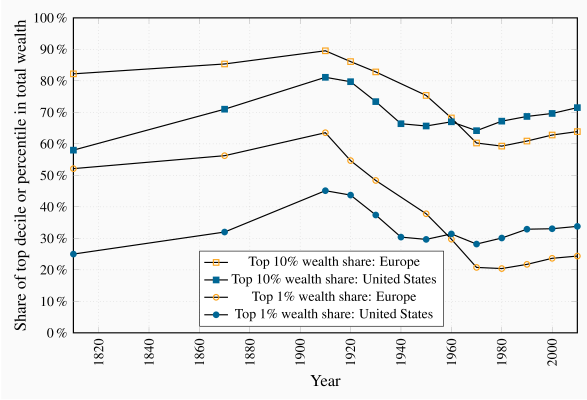
as it was about 1900. Figure 13.5 (Piketty 10.6)
above is borrowed from his web site. Wealth was more unequally distributed
in Old World Europe than New World America a century ago, but this
relativity has since been reversed. A great transformation in the wealth
holding pattern of societies in the twentieth century took the form of the
emergence of a 'patrimonial middle class', by which he means the emergence
of substantial wealth holdings on the part of that 40% of the population
below the top decile. This development is noteworthy, but Piketty warns that
the top percentiles of the wealth distribution may be on their way to
controlling a share of all wealth close to their share in the early years of
the twentieth century. He illustrates that two elements are critical to this
prediction; first is the rate of growth in the economy relative to the
return on capital, the second is inheritances.
To illustrate: Imagine an economy with very low growth, and where the owners
of capital obtain an annual return of say 5%. If the owners merely maintain
their capital intact and consume the remainder of this 5%, then the pattern
of wealth holding will continue to be stable. However, if the holders of
wealth can reinvest from their return an amount more than is necessary to
replace depreciation then their wealth will grow. And if labour income in
this economy is almost static on account of low overall growth, then wealth
holders will secure a larger share of the economic pie. In contrast, if
economic growth is significant, then labour income may grow in line with
income from capital and inequality may remain stable. This summarizes
Piketty's famous (r–g) law – inequality depends upon the difference
between the return on wealth and the growth rate of the economy. This
potential for an ever-expanding degree of inequality is magnified when the
stock of capital in the economy is large.
Consider now the role of inheritances. That is to say, do individuals leave
large or small inheritances when they die, and how concentrated are such
inheritances? If individual wealth accumulation patterns are generated by a
desire to save for retirement and old age – during which time individuals
decumulate by spending their assets – such motivation should result in small
bequests being left to following generations. In contrast, if individuals
who are in a position to do so save and accumulate, not just for their old
age, but because they have dynastic preferences, or if they take pleasure
simply from the ownership of wealth, or even if they are very cautious about
running down their wealth in their old age, then we should see
substantial inheritances passed on to the sons and daughters of these
individuals, thereby perpetuating, and perhaps exacerbating, the inequality
of wealth holding in the economy.
Piketty shows that in fact individuals who save substantial amounts tend to
leave large bequests; that is they do not save purely for life-cycle
motives. In modern economies the annual amount of bequests and gifts from
parents to children falls in the range of 10% to 15% of annual GDP. This
may grow in future decades, and since wealth is highly concentrated, these
bequests in turn are concentrated among a small number of the following
generation – inequality is transmitted from one generation to the next.
As a final observation, if we consider the distribution of income and wealth
together, particularly at the very top end, we can see readily that a
growing concentration of income among the top 1% should ultimately
translate itself into greater wealth inequality. This is because
top earners can save more easily than lower earners. To compound matters, if
individuals who inherit wealth also tend to inherit more human capital from
their parents than others, the concentration of income and wealth may become
yet stronger.
The study of distributional issues in economics has probably received too
little attention in the modern era. Yet it is vitally important both in
terms of the well-being of the individuals who constitute an economy and in
terms of adherence to social norms. Given that utility declines with
additions to income and wealth, transfers from those at the top to those at
the bottom have the potential to increase total utility in the economy.
Furthermore, an economy in which justice is seen to prevail—in the form of
avoiding excessive inequality—is more likely to achieve a higher degree of
social coherence than one where inequality is large.
Key Terms
Human capital is the stock of expertise accumulated by a worker that determines future productivity and earnings.
Age-earnings profiles define the pattern of earnings over time for individuals with different characteristics.
Education premium: the difference in earnings between the more and less highly educated.
On-the-job training improves human capital through work experience.
Firm-specific skills raise a worker's productivity in a particular firm.
General skills enhance productivity in many jobs or firms.
Signalling is the decision to undertake an action in order to reveal information.
Screening is the process of obtaining information by observing differences in behaviour.
Discrimination implies an earnings differential that is attributable to a trait other than human capital.
Lorenz curve describes the cumulative percentage of the income distribution going to different quantiles of the population.
Gini index: a measure of how far the Lorenz curve lies from the line of equality. Its maximum value is one; its minimum value is zero.
Exercises for Chapter 13
Georgina is contemplating entering the job market after graduating from high school. Her future lifespan is divided into two phases: An initial one during which she may go to university, and a second when she will work. Since dollars today are worth more than dollars in the future she discounts the future by 20%, that is the value today of that future income is the income divided by 1.2. By going to university and then working she will earn (i) -$60,000; (ii) $600,000. The negative value implies that she will incur costs in educating herself in the first period. In contrast, if she decides to work for both periods she will earn $30,000 in the first period and $480,000 in the second.
If her objective is to maximize her lifetime earnings, should she go to university or enter the job market immediately?
If instead of discounting the future at the rate of 20%, she discounts it at the rate of 50%, what should she do?
Imagine that you have the following data on the income distribution for two economies.
|
| Quintile share of total income |
|
First quintile | 4.1 | 3.0 |
|
Second quintile | 9.6 | 9.0 |
|
Third quintile | 15.3 | 17.0 |
|
Fourth quintile | 23.8 | 29.0 |
|
Fifth quintile | 47.2 | 42.0 |
|
Total | 100 | 100 |
On graph paper, or in a spreadsheet program, plot the Lorenz curves corresponding to the two sets of quintile shares. You must first compute the cumulative shares as we did for Figure 13.3.
Can you say, from a visual analysis, which distribution is more equal?
The distribution of income in the economy is given in the table below. The first numerical column represents the dollars earned by each quintile. Since the numbers add to 100 you can equally think of the dollar values as shares of the total pie. In this economy the government changes the distribution by levying taxes and distributing benefits.
|
Quintile | Gross income $m | Taxes $m | Benefits $m |
|
First | 4 | 0 | 9 |
|
Second | 11 | 1 | 6 |
|
Third | 19 | 3 | 5 |
|
Fourth | 26 | 7 | 3 |
|
Fifth | 40 | 15 | 3 |
|
Total | 100 | 26 | 26 |
Plot the Lorenz curve for gross income to scale.
Now subtract the taxes paid and add the benefits received by each quintile. Check that the total income is still $100. Calculate the cumulative income shares and plot the resulting Lorenz curve. Can you see that taxes and benefits reduce inequality?
Consider two individuals, each facing a 45 year horizon at the age of 20. Ivan decides to work immediately and his earnings path takes the following form: Earnings =20,000+1,000t–10t2, where the t is time, and it takes on values from 1 to 25, reflecting the working lifespan.
In a spreadsheet enter values 1... 25 in the first column and then compute the value of earnings in each of the 25 years in the second column using the earnings equation.
John decides to study some more and only earns a part-time salary in his first few years. He hopes that the additional earnings in future years will compensate for that. His function is given by 10,000+2,000t–12t2. In the same spreadsheet compute his annual earnings for 25 years.
Plot the two earnings functions you have computed using the 'charts' feature of Excel. Does your graph indicate that John passes Ivan between year 10 and year 11?
In the short run one half of the labour force has high skills and one half low skills (in terms of Figure 13.2 this means that the short-run supply curve is vertical at 0.5). The relative demand for the high-skill workers is given by  , where W is the wage premium and f is the fraction that is skilled. The premium is measured in percent and f has a maximum value of 1. The W function thus has vertical and horizontal intercepts of
  .
.
Illustrate the supply and demand curves graphically, and illustrate the skill premium going to the high-skill workers in the short run by determining the value of W when f=0.5.
If demand increases to  what is the new premium? Illustrate your answer graphically.
Consider the foregoing problem in a long-run context, when the fraction of the labour force that is high-skilled is more elastic with respect to the premium. Let this long-run relative supply function be  .
.
Graph this long-run supply function and verify that it goes through the same initial equilibrium as in Exercise 13.5.
Illustrate the long run and short run on the same diagram.
What is the numerical value of the premium in the long run after the increase in demand? Illustrate graphically.