Explore the way that income and wealth inequality are measured
Analyze two ways of measuring the aggregate output of an economy
Examine two critiques of national income accounting
Define the labor force and the unemployment rate
Investigate the two primary methods of measuring the aggregate price level
Explain the meaning of the inflation rate
Inspect historical movements of the key macroeconomic variables over time
In Part II, we investigated many theories that are regarded as microeconomic theories because they concentrate on individual consumers, workers, savers, and business enterprises. In Part III, we turn our attention to macroeconomic theories that concentrate on much broader changes in the economy, including changes in the behavior of households, governments, industries, foreign nations, and social classes. These theories use different economic variables than microeconomic theories because the subject matter is so much broader. To understand these theories then, it is necessary first to discuss how macroeconomic variables are measured. This chapter thus concentrates entirely on the issue of macroeconomic measurement and will set the stage for all the theories that we explore in Part III. The chapter discusses how to measure poverty, income inequality, wealth inequality, aggregate output, the labor force, the unemployment rate, the aggregate price level, and the rate of inflation. After each macroeconomic variable is defined and the method of its measurement is described, its historical pattern is considered. The historical observations will also point us in the direction of interesting questions that can only be answered with the help of the theoretical frameworks that are developed in later chapters. Also in this chapter, we will consider two important critiques of national income accounting, which is important because it shows that disagreements within economics are not confined to the realm of theory but also arise around questions of measurement.
The Measurement of Poverty
The well-being of a nation depends on many factors. Neoclassical economists argue that people have unlimited wants. They do not draw a clear distinction between wants and needs. The lack of this distinction in neoclassical theory is one source of disagreement between neoclassical and heterodox economists. Heterodox economists sometimes argue that basic needs for food, clothing, medical care, and housing are fundamentally different from preferences for fine clothes, jewelry, and expensive works of art. It is not simply the strength of the preference, according to this heterodox view, but the nature of the preference that separates needs from wants.
Because this textbook takes heterodox approaches seriously, it will approach the subject of macroeconomic measurement in a way that sharply deviates from most neoclassical economics textbooks. Neoclassical economics textbooks generally begin the discussion of macroeconomic measurement with an explanation of how the total output of a nation is measured. Goods and services of all types are lumped together according to their market values and no effort is made to distinguish between goods and services that fulfill basic human needs and the goods and services that are desirable but not essential for human life. To take the heterodox perspective seriously then, this chapter acknowledges a distinction between basic needs and inessential wants. It does so by starting with poverty measurement as a measure of the well-being of a nation. That is, the welfare of a nation’s people is evaluated according to how well the population meets its basic needs.
The U.S. Census Bureau is the government body responsible for the measurement of poverty in the United States. It uses an official poverty measure and a supplementary poverty measure and each is based on “estimates of the level of income needed to cover basic needs.”[1] To calculate the official poverty rate, the U.S. Census Bureau calculated the amount of money that a household spent on food in 1963 and then tripled it while adjusting it for inflation in later years and for differences in family size, family composition, and age of the householder.[2] This amount of money income is called the poverty threshold. According to the U.S. Census Bureau, 48 different poverty thresholds exist because families are so different according to size and age.[3] In any case, the measure suggests that a household needs to spend a full 1/3 of its income on food, leaving 2/3 for all other expenses.
Once the poverty threshold is known, it is possible to determine whether a family lives in poverty. The U.S. Census Bureau calculates the Ratio of Income to Poverty by dividing total family income by the poverty threshold as follows:[4]
The following definitions are used:
In words, if the ratio of income to poverty is less than one, then the family is living in poverty because its income is below the poverty threshold. If the ratio of income to poverty is greater than or equal to one but less than 1.24, then the family is living at a near poverty level because its income has not reached 125% of the poverty threshold. Finally, if the ratio of income to poverty is less than or equal to half of the poverty threshold, then the family is living in deep poverty.[5]
The U.S. Census Bureau also provides a helpful example to illustrate the calculation.[6] A similar example is provided below:
Suppose that a family of five earns $28,000 per year. The 2016 poverty threshold for a family of five was $29,360. The ratio of income to poverty in this case is $28,000/$29,360 = 0.9537. Because the ratio of income to poverty is less than one but greater than 0.50, the family is living in poverty although not in deep poverty. The U.S. Census Bureau also defines the income deficit (if negative) or the income surplus (if positive) as the difference between family income and the poverty threshold as follows:[7]
In other words, the family of five would require $1,360 to meet the threshold and move from poverty to near poverty.
Finally, the official poverty rate refers to the percentage of the population that lives below the poverty threshold. Over time, the U.S. official poverty rate has fluctuated as shown in Figure 12.1.
As Figure 12.1 shows, the U.S. poverty rate fell significantly during the economic expansion of the 1960s but rose during the recessions in the early 1980s and early 1990s. It also declined during the economic expansion of the 1990s but rose again after the 2001 recession and even more during the Great Recession. The poverty rate thus seems to follow a somewhat countercyclical movement, which means that it rises during recessions and falls during expansions.
The official poverty rate has been in use for a half century, but it has some serious shortcomings. The Institute for Research on Poverty at the University of Wisconsin-Madison has summarized the most common criticisms of the official poverty measure, a few of which are listed below:[8]
It only represents a headcount, but it does not measure “the depth of economic need.”
It omits taxes and medical expenses and does not include noncash income like food assistance.
It does not account for geographic differences in the cost of living throughout the U.S.
We can also add to this list the omission of many people such as those in prison or nursing homes, homeless people, and foster children under age 15.[9]
Because of the problems with the official poverty measure, by 2008, New York City and other cities were developing their own poverty measures.[10] The official poverty rate has become increasingly irrelevant because as Rebecca Blank explains, food prices have fallen significantly and housing and energy prices have risen.[11] The poverty threshold has become less meaningful as a result. Resolving these issues is of great importance because food stamp eligibility depends on it, and some federal block grants to states depend on state poverty rates.[12]
To address these issues, the U.S. Census Bureau introduced a supplemental poverty measure in 2011. The supplemental poverty measure offers “a more complex statistical understanding of poverty by including money income from all sources, including government programs, and an estimate of real household expenditures.”[13] The supplemental poverty measure is also linked to poverty thresholds but the thresholds tend to be higher than the official poverty thresholds.[14] The new measure has other benefits, such as its ability to demonstrate the impact of specific safety net programs on poverty rates.[15] Nevertheless, as its name suggests, the supplemental poverty measure has not yet replaced the official poverty measure. Instead, it continues to be used as an additional tool for the measurement of poverty.
The Measurement of Income Inequality and Wealth Inequality
In neoclassical economic theory, a person’s well-being is asserted to depend only on his own consumption level with greater levels of consumption representing greater amounts of satisfaction or utility. Heterodox economists often criticize this way of thinking because it ignores the impact that unequal consumption levels may have on human well-being. This section is also committed to taking the heterodox perspective seriously and so will consider the two measures of well-being that are most relevant in this connection: measures of income inequality and wealth inequality.
The amount of inequality that exists in society directly affects human well-being. Those with lower incomes or less wealth experience envy and feel dissatisfied with what they have. Those feelings arise because others have more and those with more often enjoy putting it on display for others to see. Those with lower incomes or less wealth may devote a great deal of time and effort trying to acquire more. They may turn to illegal activities such as illegal drug sales or burglary to accumulate more and overcome such feelings. Depression and anxiety may also be a result of slipping behind others in the race to accumulate material possessions. To overcome these feelings, many people turn to shortcuts such as gambling and playing the lottery. Because such solutions rarely lead to lasting gains for people, the pressure to find a solution becomes that much greater.
On the other hand, those with high incomes or great wealth become the subjects of envy and are placed in a defensive position. They must devote effort to justifying their high incomes or great wealth. Economic theory may serve this end insofar as it provides theoretical explanations for the incomes and wealth levels that emerge in capitalist societies. Nevertheless, many with great incomes and wealth will put it on display so that it becomes an object of envy for others. Such displays are what Thorstein Veblen called conspicuous consumption and might include expensive artwork, mansions, boats, sportscars, jewelry, and vacations. Others with great income and wealth separate themselves from the rest of the population in gated communities or high-rise apartments.
At all levels, the preoccupation with having more leads people to forget about other aspects of life such as family relationships, which often suffer because of the focus on material gain. The beauty of nature and the joy of hobbies are also forgotten as people seek ways to accumulate more wealth and to elevate themselves above their peers. Great wealth can also lead to the exploitation of labor-power from a Marxian perspective as capital is put in motion to produce surplus value. Because income inequality and wealth inequality are so important to our economic well-being, it makes sense to explore the primary method of measuring them.
One method of measuring income inequality is to use a statistic called the quintile ratio. The quintile ratio is the ratio of the income of the top fifth of the population to the income of the bottom fifth of the population. The ratio ignores the middle 3/5 of the population, but it helps us to see just how much of a spread exists between the top income earners and the bottom income earners. The higher the quintile ratio, the higher is the degree of income inequality. For example, a quintile ratio of 5 implies that the top income earners have five times the income of the bottom income earners. If the quintile ratio rises to 6, then the top income earners have six times the income of the bottom income earners, and inequality has increased.
Table 12.1 shows the quintile ratios for several countries in 2018.
Table 12.1 arranges the countries from the least equal to the most equal as reflected in the falling quintile ratios as you move down the column. In Table 12.1, Colombia has the highest degree of income inequality, and Norway has the least income inequality of the countries in the table.Figure 12.2 shows an example of a Lorenz Curve.
In Figure 12.2, the first 25% of the population holds 15% of the income. The first 50% of the population holds 20% of the income. The first 75% of the population holds 45% of the income. Finally, 100% of the population holds 100% of the income.
The 45-degree line has a special role to play relative to the Lorenz Curve. The 45-degree line represents perfect equality. It shows that 25% of the population holds 25% of the income. 50% of the population holds 50% of the income. 75% of the population holds 75% of the income. 100% of the population holds 100% of the income. Therefore, the further away from the 45-degree line the Lorenz Curve is, the more income inequality is implied.
It is possible to measure the extent of the deviation of the Lorenz Curve from the 45-degree line. Two areas have been marked in the graph: Area A and Area B. When Area A is larger and Area B is smaller, the Lorenz Curve is further from the 45-degree line, and more income inequality exists. When Area A is smaller and Area B is bigger, then the Lorenz Curve is closer to the 45-degree line and less income inequality exists. To measure the extent to which the Lorenz Curve deviates from the 45-degree line, economists use something called the Gini Coefficient. The Gini Coefficient is calculated as Area A divided by the sum of Areas A and B:
The extreme values of the Gini Coefficient are zero and one. When the Lorenz Curve coincides with the 45-degree line, Area A is equal to zero and so the Gini Coefficient is equal to zero, which indicates perfect income equality. When the Lorenz Curve perfectly coincides with the lower right angle, Area B is equal to zero and so the Gini Coefficient is equal to 1, which indicates perfect income inequality. Perfect income inequality means that one person has all the income and the rest of the population has zero income. In general, the Gini Coefficient will fall somewhere in between these extremes and is usually between 0.20 and 0.50. Extreme cases are a bit higher or lower.
Table 12.2 shows estimates of the Gini Coefficient for several years for the United States.
Table 12.2 shows clearly that the level of income inequality in the U.S. has worsened over time. It is also possible to create a Lorenz Curve to represent the distribution of wealth and a Gini Coefficient to measure the extent of wealth inequality. In the U.S., the distribution of wealth has been much more unequal than the distribution of income. Figure 12.3 places Lorenz Curves representing the distribution of income and the distribution of wealth on the same graph.
Because the wealth distribution Lorenz Curve is further from the 45-degree line than the income distribution Lorenz Curve, we can infer that the distribution of wealth is more unequal than the distribution of income. This inequality in the distribution of wealth is only expected to worsen. According to a new analysis that the House of Commons Library conducted, if the current pattern continues, then the top 1% of the global population will own 64% of global wealth by 2030.[16]
The Measurement of Aggregate Output
We now turn to the primary measure of macroeconomic performance among neoclassical economists, which is a measure of the aggregate output of the economy that is called Gross Domestic Product(GDP). GDP is intended to give us a sense of the size of the economic pie of a nation. It is one of the major components of the National Income and Product Accounts (NIPA). The U.S. Bureau of Economic Analysis (BEA) within the U.S. Department of Commerce maintains the NIPA and publishes quarterly estimates of U.S. GDP.
To be precise, GDP represents the total market value of all final goods and services produced in a year within the national boundaries of a nation. Final goods and services refer to goods and services that are sold for final consumption. It should also be noted that GDP is a flow variable because it is measured per period such as a year. Figure 12.4 shows a production possibilities frontier (PPF) for a simple economy with just two final goods: apples and oranges.
Figure 12.4 shows two combinations of apples and oranges that the economy produces in two different years. In 2001, it produces 400 apples and 300 oranges. In 2002, it produces 300 apples and 400 oranges. The reader should recall that the quantities of each good are measured in real terms (i.e., so many apples and so many oranges). It is not meaningful to add up all the apples and oranges in a year because they are qualitatively different goods. Even if we are satisfied adding together different types of fruit, if the goods produced in this economy included apples and automobiles, then adding these goods together would really make no sense. In general, the fact that differences exist among the units in which each good is measured prevents us from adding together the real quantities.
Neoclassical economists resolve this problem through the assignment of weights to each good, which makes possible their conversion into a common unit and their aggregation. The natural weights to use are the market prices of the goods. More valuable goods, like automobiles, will be assigned greater weights and less valuable goods, like apples, will be assigned smaller weights. Table 12.3 adds price information to our example of an economy that produces apples and oranges.
If we multiply each real quantity of a good by the market price of the good, then we obtain a dollar value of that good for the year. We then add the dollar values of apples and oranges for that year and we obtain the aggregate output or GDP for this simple economy. This measure of aggregate output makes it possible for us to compare the size of the economic pie across two years. Since GDP has risen from $775 to $800, we conclude that GDP has risen from 2001 to 2002. Without the common metric that money provides, it would not be possible to draw any conclusions about the change in aggregate output between 2001 and 2002.
It is important to ask why economists limit the measurement of aggregate output to final goods and services. The values of intermediate goods, or goods that become part of other goods during production, are specifically excluded from the GDP calculation. The reason for the exclusion of the values of intermediate goods is that their inclusion would lead to a problem referred to as double counting. For example, suppose that a tire manufacturer purchases rubber from a supplier at a price of $150. The tire is then manufactured and sold to an automobile manufacturer for $250 who uses it to produce an automobile. The automobile is then sold to a consumer for $20,000. The automobile is the final good in this scenario, and the rubber and tire are intermediate goods. Therefore, only the value of the automobile is counted as part of GDP and the values of the rubber and the tire are intentionally omitted from the calculation. Why? The reason is that the $20,000 price of the automobile includes the value of the tire, which includes the value of the rubber. The supplier has added $150 to the value of the rubber through its production process (assuming it is the first stage of production). The tire manufacturer then adds another $100 to the value of the rubber, which results in a tire worth $250. The automobile manufacturer then adds additional value to the tire because it is now a part of a finished automobile. Let’s suppose that $400 is the value of the tire, which makes up part of the $20,000 sale price of the automobile. The automobile manufacturer has thus added another $150 of value to the tire. The reason for excluding the values of the rubber and the tire should be clear. The $400 tire, which is part of the sale price of the automobile, already includes the value of the rubber sold to the tire manufacturer and the value of the tire sold to the automobile manufacturer. If we count the value of the rubber and the value of the tire in the calculation of GDP, then we will be counting the value of the rubber three times and the value of the tire two times! To avoid multiple counting, we only add the value of the final good or service when calculating GDP. An alternative method is to add up the values added at each stage of production. In this case, we would add $150 for the value of the rubber, $100 for the value that the tire manufacturer adds, and $150 for the value that the automobile manufacturer adds to the tire due to the production of the finished automobile. Of course, we would then need to add the remaining $19,600 of value that the auto manufacturer adds with labor and other component parts to obtain the $20,000 contribution to GDP. Either of the two methods avoids double counting, and arguably results in a better approximation of the contribution of these goods to the national economic pie.
In addition to the exclusion of the values of intermediate goods, several other exclusions apply to the calculation of GDP. National income accountants exclude government transfer payments. Government transfer payments include social security benefits and public assistance of all kinds. Because they do not represent a payment for a real good or service, they do not count in the calculation of GDP. National income accountants also exclude private transfer payments from the calculation of GDP. Private transfer payments include monetary gifts and charitable donations. When a donor makes a charitable donation, she typically receives a letter from the charity thanking her for the contribution. The letter also states that the organization did not grant any goods or services in exchange for the donation. Because the donation does not reflect any current production of goods or services, GDP should not include it. National income accountants also exclude sales and purchases of financial assets, such as stocks and bonds. It is possible to link stocks and bonds to production processes, but these assets only represent claims to the assets of a corporation and so are not included in GDP. Finally, used goods are also excluded from the GDP calculation because the current year GDP or the previous year’s GDP includes the values of the goods when sellers sold them the first time. For example, the sale of a 2014 Ford Escape in 2018 should not be included in the GDP for 2018 because the 2014 GDP already included it. The sale of used goods represents the redistribution of existing output rather than the production of new output. For that reason, the GDP calculation excludes the values of used goods.
From a conceptual perspective, two methods exist for thinking about the measurement of aggregate output. The two methods stem from what is an identity in neoclassical economics, namely that income and expenditure are always equal as shown in Figure 12.5.
If I purchase that new 2014 Ford Escape for $20,000 in 2014, then we can think about my expenditure of $20,000, which is equal to the value of that final good. We can also think about it from the perspective of the dealer who receives an income of $20,000 when she sells the automobile. At a macroeconomic level, whether we add up all the expenditures on final goods or whether we add up all the incomes received from the sale of final goods, we should obtain the same measure of aggregate output. This result must hold true because of the income-expenditure identity.
To delve deeper into the expenditures approach to the measurement of GDP, national income accountants divide aggregate expenditures into four major categories: personal consumption expenditures (C), gross private domestic investment (I), government purchases (G), and net exports (Xn). If we add together these four values, we obtain GDP as follows:
Personal consumption expenditures include expenditures on durable goods, nondurable goods, and services. The consumption of durable goods typically requires more than three years, and includes such items as automobiles and household appliances. The consumption of nondurable goods typically requires less than three years, and includes such items as food, clothes, and fuel. Finally, services include nontangible commodities like legal services, medical services, and childcare.
Gross private domestic investment includes several types of expenditure as well. Expenditures on final capital goods that businesses incur are included in this category. When a business purchases a machine, for example, it is considered a final capital good because the machine does not become physically incorporated into another product. Its use in the production process is its final use. One potential complication here is that the value of a final capital good is gradually transferred to the value of the good that it is used to produce. As the machine depreciates, that value must pass to the value of the final product because it represents a cost of production. Later in this section, we will consider how national income accountants address this issue.
Residential fixed investment is another type of investment expenditure in the national income accounts. It refers to all expenditures incurred in the purchase of newly constructed homes. When homes are resold, they are not included in the GDP calculation because that would represent double counting. Previous home construction was already counted once when the homes were sold for the first time. The reader might find it odd that homes are considered an investment expenditure rather than a consumption expenditure. The reason is that investment expenditures are a positive contribution to the nation’s stock of capital and houses may be thought of as capital goods. In neoclassical theory, capital goods are goods used to produce other goods. In the case of housing, houses produce a flow of services over time. That is, a home creates a space for a person to live that can benefit that person for many years. The house thus contributes to the production of this service and so the house may be thought of as a capital good. Business fixed investment is another category of investment expenditure in the national income accounts. It refers to expenditures incurred in the construction of new factories, production plants, and office buildings. Business investments of this kind also make possible the production of other goods and services and so represent an increase in the nation’s capital stock.
Inventory investment is another type of investment expenditure in the national income accounts. It is calculated as changes in inventories in a year. Business inventories expand when firms have unsold goods at the end of a calendar year. They store these goods with the hope of selling the goods in the next year. Even though these goods are not sold to the public, they do represent new production of final goods and should be counted in GDP. Hence, national income accountants include new additions to inventories when calculating GDP. It is as if the businesses purchase the goods even though no money changes hands. On the other hand, some businesses will sell goods in the current year that were produced in a previous year and became part of their business inventories in that previous year. Because these goods were already counted as part of a previous year’s GDP since they represented additions to inventories at that time, these sales should be subtracted in the calculation of GDP. One might wonder why they need to be subtracted as opposed to simply ignored. They must be subtracted because when personal consumption expenditures are calculated, they include all goods and services sold to consumers, which might include goods that were produced in a previous year and became part of business inventories at that time. The subtraction at this stage allows national income accountants to remove them from the calculation of GDP. Inventory investment is thus calculated as follows:
It is possible for inventory investment to be positive if new additions to inventories outweigh reductions in inventories in a year. It might also be equal to zero if the additions and reductions perfectly balance. Finally, it might be negative, if reductions in inventories are so large that they exceed new additions to inventories. In the last case, negative inventory investment will cause GDP to be smaller.
At this point it might be helpful to consider how the nation’s stock of private capital changes over time.[17] The nation’s private capital stock refers to all the privately-owned machinery, homes, factories, office buildings, production plants, apartment buildings, etc. at a specific point in time. Gross private domestic investment causes the private capital stock to grow. At the same time, depreciation causes the private capital stock to contract. Depreciation refers to the gradual wearing out of capital over time due to use or lack of use. The relationship between gross investment and depreciation in a year determines the net impact on the private capital stock. Gross investment may be thought of as an inflow and depreciation may be thought of as an outflow relative to the private capital stock. Figure 12.6 shows these relationships.
Since gross investment and depreciation cause annual changes in the size of the private capital stock, they are flow variables. The private capital stock is obviously a stock variable because it is measured as of a point in time. If gross investment exceeds depreciation, then the private capital stock expands. That is, more is added to the private capital stock than is depleted. If gross investment is below depreciation, then the private capital stock contracts. That is, more of the private capital stock is wearing out than is being replaced. If gross investment and depreciation are equal, then the private capital stock remains constant for that year.
Returning to the components of aggregate expenditure that are used to measure GDP, the third type is government purchases of final goods and services. Federal, state, and local governments purchase consumer goods and services such as office supplies and computers for use in government buildings. Governments also make investment expenditures when they build new roads, bridges, schools, and office buildings. Because all these purchases represent purchases of final goods and services, we should include them in our calculation of GDP.
The final component of aggregate spending that is used to calculate GDP is net exports. Net exports are the difference between exports and imports (X – M). It is also referred to as the balance of trade or simply as the trade balance. It should be obvious why we add exports in the calculation of GDP. GDP is supposed to include the values of all domestically produced final goods and services in a year. When final goods and services are produced and exported, the expenditure that foreign buyers incur should be included in GDP. Imports of final goods and services, on the other hand, are produced outside the territorial boundaries of the nation and so should be included in the GDPs of foreign nations. The reader might wonder why we subtract imports in the calculation of GDP rather than simply ignoring them altogether. As with spending on goods produced in previous years, personal consumption expenditures might include spending on imported goods and services. No effort is made to exclude imported goods and services from that component of aggregate expenditure. Therefore, we subtract imports at this stage to ensure that they are not included in our GDP measure. Similarly, government purchases of final goods and services and business purchases of final capital goods might include purchases of imported goods. The subtraction of imports also allows us to exclude those values from our GDP calculation.
Because imports are subtracted in the calculation of net exports, it is possible for net exports to be negative. When a nation’s imports exceed its exports, then we say that a trade deficit exists and net exports are negative. When a nation’s exports exceed its imports, then we say that a trade surplus exists and net exports are positive. When the nation exports and imports the same amount, then we say that balanced trade exists and net exports are equal to zero.
Table 12.4 shows the numerical figures for each of the major components of aggregate expenditure in 2017.
The sum of personal consumption expenditures, gross private domestic investment, government purchases, and net exports is equal to GDP for that year. As Table 12.4 shows, GDP for 2017 was equal to $19.3906 trillion. In general, personal consumption expenditures tend to be about 2/3 (or about 66.67%) of GDP. This statistic is a frequently quoted statistic in the economic news of the nation. It is often stated that consumer spending makes up 2/3 of the economy. When people make this claim, they have in mind 2/3 of GDP. Government purchases are usually about 20% of GDP. Investment spending is typically about 10-15% of GDP. Net exports tend to be the smallest component of aggregate spending at about 3% and have been negative in recent decades. The percentages shown in Table 12.4 are approximately at these levels. Also, the reader should notice that the U.S. trade deficit is reflected in the negative value of net exports.
We next turn to the income approach to the measurement of GDP. The income approach adds up all the different flows of income that result from the sale of final goods and services. The largest income flow is compensation for American employees (i.e., wages and salaries). That is, when goods and services are sold, part of the revenue is used to pay employees of businesses. Rental income for American landlords is another major income category. Part of the revenue from the sale of final goods and services goes to pay rent for properties that are used in production. Interest income for American moneylenders is a third major income category. When final goods and services are sold, part of the revenue must be used to pay interest on loans. Finally, profit income for American businesses represents a major income flow. Part of the revenue from the sale of final goods and services businesses appropriate as profits. A portion of the profit income is for unincorporated businesses like sole proprietorships (one owner) and partnerships (multiple owners). Such businesses face unlimited liability. That is, if the business fails, then the owners’ personal assets must be used to pay business debts. The rest of the profit income consists of corporate profits or the profits of incorporated business enterprises. Corporations issue and sell stock to the public. These business enterprises enjoy limited liability. If the firm fails, only the corporation’s assets may be used to pay the firm’s debts. The losses for the owners will be limited to the amount of money capital they contributed to the business. Corporate profits are subject to federal and state corporate income taxes and so a portion will be paid to the federal and state governments. Another portion may be distributed as dividends to the shareholders, who are the owners of the corporations. Finally, a third portion of corporate profits might be reinvested in the business and constitute what are called retained earnings because they are neither paid as taxes nor distributed to owners.
Three additional income flows must be considered before we arrive at our measure of GDP. When final goods and services are sold, a part of the revenue must be used to pay taxes on the sale. Taxes on production and imports include taxes, such as state sales taxes, excise taxes, and import tariffs. These income flows pass to federal and state governments. Another income flow is used to replace worn out capital. When businesses sell final goods and services, they set aside a portion of the revenue to repair and replace capital goods that have been used in production. A fund that represents the depreciation of the capital stock is thus another income flow that must be included in the GDP calculation.
The final income flow that must be included in the GDP calculation is a measure that national income accountants refer to as net foreign factor income. To understand this measure, we must recall that all compensation for employees, rental income, interest income, profit income and taxes on production and imports that were previously discussed flow to American citizens, businesses, and governments. National income is the sum of all these incomes flows as expressed below:
That is, whether American workers and businesses are working and operating in the United States or in the rest of the world, their incomes are counted in these income measures. Because GDP measures all the income received within the territorial boundaries of the nation, to calculate U.S. GDP using the income approach, we must adjust aggregate income to account for the fact that some Americans are earning income abroad while some foreigners are earning income in the U.S. Figure 12.7 provides a diagram that shows why this adjustment must be made.
In Figure 12.7, the income that foreign citizens and businesses earn in the U.S. is denoted as F1, and the income that American citizens and businesses earn outside the U.S. is denoted as A2. Similarly, the income that American citizens and businesses earn in the U.S. is denoted as A1, and the income that foreign citizens and businesses earn outside the U.S. is denoted as F2. To calculate U.S. GDP, we need to subtract A2 and add F1 when starting with U.S. national income. This adjustment will allow us to calculate all the income earned within the geographical boundaries of the United States. We can now calculate net foreign factor income as follows:
To move us closer to the calculation of U.S. GDP, we need to subtract net foreign factor income from U.S. national income. Subtracting net foreign factor income will remove the income of Americans working abroad and add the income of foreigners working in the U.S. The final adjustment to national income is the addition of depreciation, which is an income flow that is not included in U.S. national income. U.S. GDP using the income approach may thus be calculated as follows:
Figure 12.7 also allows us to see that net foreign factor income is the difference between Gross Domestic Product (GDP) and Gross National Product (GNP). GNP was used more widely in the past in studies of aggregate output. It includes all the output produced and all the income earned by U.S. citizens whether working in the U.S. or abroad. In other words, GNP would equal A1+A2 in Figure 12.7, and so it would not include F1. GDP, on the other hand, would equal A1+F1 but it would not include A2. The shift of focus from GNP to GDP in the U.S. occurred in the 1990s and makes sense in an increasingly globalized world where location seems more important than citizenship when thinking about contributions to the total production of the economy.
The income and expenditures approaches to the measurement of GDP should lead to the same numerical result because the approaches are based on the income-expenditure identity. The project of adding all the expenditure in the economy and all the income earned is such a massive project, however, that errors are inevitable. Because the two calculations do not match in practice, national income accountants include an item called statistical discrepancy to ensure that the two calculations are the same after accounting for the errors that arise from data collection. Table 12.5 shows the figures for U.S. GDP in 2017 using the income approach.
A value for statistical discrepancy has been included so that the GDP calculation is the same (aside from rounding error) as the calculation using the expenditures approach in Table 12.4. To summarize the two approaches to GDP measurement in a single diagram, consider Figure 12.8.
Figure 12.8 shows how the four major categories of aggregate expenditure generate incomes for workers, landlords, savers, and businesses (profits and depreciation funds) working and operating in the U.S. as well as U.S. federal, state, and local governments.
National income accountants use additional measures of macroeconomic performance. Starting with GDP, we can work backwards, in a sense, to obtain these other measures. For example, if we subtract depreciation from GDP, we obtain a measure called Net Domestic Product (NDP), which is calculated as follows.
NDP shows us the value of the final goods and services produced in a year after we account for the depreciation of the capital stock. This measure addresses an issue raised earlier in this chapter regarding the possibility of double counting that results from the inclusion of final capital goods as an investment expenditure in the calculation of GDP. When a final capital good is used, it depreciates and adds value to the good that it is used to produce. If we count the full value of the final capital good in GDP and the value that it adds to final goods during the year, then double counting will occur. By subtracting depreciation, we eliminate the double counting problem. In 2017, U.S. NDP was calculated as follows:
We can also reconstruct U.S. national income if we add net foreign factor income to U.S. NDP. This addition will add the incomes of Americans working abroad and subtract the incomes of foreigners working in the U.S.
The GDP measure is a helpful way to think about aggregate output and aggregate income. Nevertheless, it is not a perfect measure. One of the problems with GDP is that it can change from year to year for reasons that do not seem to correspond with a change in the production of real final goods and services. For example, because prices are used as weights in the GDP measure, if all prices increase from one year to the next, then GDP will rise even if the real quantities produced have not changed. Let’s again consider a simple economy that only produces apples and oranges. Table 12.6 shows the quantities of each good and their prices for three different years.
Nominal GDP is calculated by multiplying prices and quantities and summing them up as explained previously. Nominal GDP refers to GDP measured in current year market prices and is the measure that we have been discussing all along. As Table 12.6 shows, nominal GDP rose between 2001 and 2003, but it rose for two reasons. One reason is the increase in real quantities of apples and oranges produced. The second reason is the rise in the prices of apples and oranges. If we want our measure of aggregate output to only capture increases in real quantities produced, then we have a problem. The problem is the result of changing prices and so the obvious solution is to fix the prices. Which prices should we use? We have market prices from three different years that we can use in our calculation. It really does not matter which set of prices we use if they are constant. Because the choice is arbitrary, we will designate one year as the base year and then use the base year prices to calculate GDP for any year.
Table 12.7 shows how GDP is calculated using constant 2001 prices.
That is, 2001 has been selected as the base year and has been used to calculate real GDP. Real Gross Domestic Product (GDP) is the measure of aggregate output using current year quantities and base year or constant prices. It should be clear that Real GDP has risen between 2001 and 2003 but the increase is much less dramatic than the increase in nominal GDP during those years. The reason, of course, is that real GDP only increases because of the increase in real quantities. Nominal GDP, on the other hand, rises due to the increase in real quantities and the rise in market prices. Because Real GDP allows us to focus on changes in real production, it is argued to be a superior measure of aggregate output.Figure 12.9 shows how real GDP has fluctuated around a long-term trend line representing economic growth between 1990 and 2017.[18]Reductions in real GDP are considered recessions and increases in real GDP are considered expansions. When real GDP reaches a local maximum, it is considered the peak of the business cycle. When real GDP reaches a local minimum, it is considered the trough of the business cycle. As a rule of thumb, economists usually regard two consecutive quarters of negative real GDP growth as a recession. Recessions vary a great deal, however, in terms of their length and intensity. They can be long and deep or short and mild. The length and intensity of expansions is also difficult to predict.Figure 12.10 represents the series of surpluses and shortages that emerge in the market and how the output of this product that is available in the market fluctuates over time.
This simple model is referred to as the cobweb model.[19] More sophisticated versions of the cobweb model show the market price gradually approaching the equilibrium price as the adjustments become smaller and begin to approach their target. Assuming many or all individual markets experience such fluctuations, an aggregation of these output fluctuations will produce macroeconomic fluctuations with corresponding fluctuations in employment. Because the explanation of business fluctuations stemming from the cobweb model is rooted in errors made by producers, it may be considered a heterodox theory of economic cycles. As we will see, however, most orthodox and heterodox explanations of business cycles emphasize other factors. Later chapters delve into the sources of these different explanations.
In addition to real GDP, economists also frequently discuss the growth rate of real GDP. The real GDP growth rate is calculated as follows:
The calculation of the real GDP growth rate between year t-1 and year t divides the change in real GDP by the real GDP of the previous year. A positive rate of real GDP growth suggests that real GDP has increased since the previous year. A negative rate of real GDP growth suggests that real GDP has fallen since the previous year. A zero rate of real GDP growth suggests that real GDP has remained the same since the previous year.
Another measure that economists use is per capita real GDP or real GDP per person. Per capita real GDP is calculated as follows:
Per capita real GDP is often considered to provide a rough measure of the standard of living in a nation. It measures real income or real output per person. The measure has a serious shortcoming, however, because it is only an average and does not tell us anything about an individual’s economic welfare. If everyone receives the same real income, then per capita real GDP tells us what that real income level is. If a great deal of income inequality exists, however, then some people will have real incomes that are far below the per capita real GDP. Other people will have real incomes that are far above the per capita real GDP. In other words, per capita real GDP tells us nothing about the distribution of income. If someone suggests that it is a rough measure of what individuals earn in real terms, then that suggestion can be very misleading.
Nevertheless, a rise in per capita real GDP gives us a sense of how much the economy has expanded over time. Figure 12.11 shows how the per capita real output has increased dramatically from 1947 to 2017.
A similar measure that uses real GDP in its calculation is real GDP per worker, which measures the average labor productivity for each member of the labor force as follows.
A higher level of real output per worker suggests higher average labor productivity. A lower level of real output per worker suggests lower average labor productivity. Again, this measure is subject to the same shortcoming in that it is only an average. Nevertheless, economists widely use both the labor productivity and per capita output measures. Economists also refer to the growth rates of real per capita income and real output per worker as measures of economic growth and productivity changes. A productivity growth slowdown began in the 1970s. The reasons for the productivity slowdown are hotly debated. Some explanations focus on the inflation that occurred in the 1970s while other explanations focus on the breakdown of the cooperative labor-management relations of the postwar period. The macroeconomic theories in the second part of this book offer explanations for such changes.
Heterodox Critiquesof National Income Accounting
Many heterodox economists are sharply critical of national income accounting. This section concentrates on two major critiques of GDP as a measure of economic well-being. The first critique is one that feminist economists have developed to draw attention to the many contributions that women make to our economic well-being that have been excluded from the calculation of GDP. The second critique involves the assertion that human happiness depends on more than the amount of goods and services that are available for consumption. We consider each critique separately.
GDP only includes the market value of all final goods and services produced within the economy during a given year. Because it only includes market values, any production that never finds its way to the market is necessarily omitted from the calculation of GDP due to the lack of a market price. One type of production that never enters the market is household production. Historically, women have been the primary producers within the home of a huge variety of goods and services, including home-cooked meals, laundry services, cleaning services, childcare, care of elderly family members, care of pets, transportation for children and the elderly, gardening and landscaping, clothing, clothing repair, and grocery shopping. The list could easily be expanded.
When people outside the home are hired to perform these services and produce these goods, the production is counted in GDP because it has a market value. When women perform these duties within the home and their families consume the goods and services, they are not counted in GDP. Consequently, an enormous amount of labor that women have performed during the past century has been completely overlooked in the national income accounts. It is the invisible nature of women’s unpaid work in the home that has been the motivation for sharp feminist critiques of GDP as a measure of economic welfare.
Some early estimates of national income in Norway and other Scandinavian countries included the value of unpaid household labor. For example, in Norway in 1943, the value of unpaid household labor was estimated to be 15% of national product.[20] As the United Nations prepared to introduce the first international standard for national accounts in 1953, however, goods and services derived from unpaid household work were excluded, which led Norway to eliminate it from its national accounts in 1950.[21]
The primary method of accounting for goods and services that do not have market values is to use imputed values. The imputed value of a good or service is based on its likely value in the market if it was sold. It can be thought of as the opportunity cost of consuming the good or service when it could be sold. The practical way to handle this problem when considering unpaid labor in the home is to assume that “an hour of market work and an hour of nonmarket work have the same value.”[22] The market wage of a substitute household worker is then used in combination with the labor time needed to produce goods and services in the home.[23] The typical choice of yardstick to arrive at the estimates of the value of household labor is extra gross wages, which are before taxes and include employers’ social security contributions.[24] A rough estimate of the value of nonmarket household production is approximately half of GDP in the industrialized countries.[25] Given how massive this contribution is, the omission of unpaid household labor in the national income accounts grossly understates our national output of goods and services.
At the same time, feminist economists recognize that many activities within the home have an intrinsic value that market values simply cannot capture.[26] To represent these intrinsic values, quality of life measures are used that include the “pursuit of good health, the acquisition of knowledge, the time devoted to fostering social relationships, [and] the hours spent in the company of relatives and friends.”[27] However we might measure the contribution of unpaid household labor, it is essential to recognize that it is women’s contribution that is mainly being overlooked in the national income accounts. In industrialized nations in recent decades, women spent about 2/3 of their total work time on unpaid nonmarket activities and 1/3 of their time on paid market activities whereas for men the shares have been reversed.[28] In developing nations, the difference between men’s and women’s shares is even greater.[29]
For an alternative measure of macroeconomic well-being, we turn to the Himalayan Mountains where Bhutan’s primary measure is something called Gross National Happiness (GNH). GNH has become a guiding light of economic policymaking in Bhutan. Since Bhutan became a democracy in 2008, its Constitution has required its leaders “to consult the four pillars of Gross National Happiness – good governance, sustainable socioeconomic development, preservation and promotion of culture, and environmental conservation – when considering legislation.”[30]
Bhutan’s rejection of GDP as a measure of economic progress goes back to 1971.[31] This Buddhist approach to economic well-being places emphasis on “the spiritual, physical, social and environmental health of its citizens and natural environment.”[32] To protect the natural environment, Bhutan has taken extraordinary measures. It is committed to remaining carbon neutral and to permanently maintaining 60% of its landmass under forest cover, which has included a ban on export logging.[33] The GNH concept has also influenced Bhutan’s system of education, which places heavy emphasis on environmental protection, recycling, and daily meditation.[34]
King Jigme Singye Wangchuck, who ruled Bhutan until 2006, coined the GNH label decades ago.[35] It is worth noting that the concept was developed in Asia rather than in western nations where material possessions have long served as the measure of well-being. Nevertheless, the concept has caught on with western leaders. In 2011, the UN General Assembly “passed a resolution inviting member states to consider measures that could better capture ‘the pursuit of happiness’ in development,” which led to the first World Happiness Report of 2012.[36] The UN uses a variety of different variables to calculate a score for each country, which serves as its index of happiness. According to the 2018 World Happiness Report, Finland is the happiest nation on the planet and the U.S. has fallen to 18th place due to crises of obesity, substance abuse, and mental health problems.[37] Although GNH has not replaced GDP as the measure of greatest interest to most economists, it has drawn public attention to the possibility that our economic welfare depends on more than the amount of final goods and services our nation produces each year.
The Measurement of the Labor Force and the Unemployment Rate
We now turn to the measurement of the labor force, employment, and unemployment. Within the U.S. Department of Labor, the Bureau of Labor Statistics (BLS) is responsible for publishing the unemployment rate each month. To understand this calculation and related measures, consider Figure 12.12, which breaks down the population into its component parts.
Figure 12.12 shows that the total population may be divided into the civilian non-institutional population and those not in the civilian non-institutional population. Those in the civilian non-institutionalpopulation are at least 16 years old and are not in institutions such as mental hospitals or prisons. Those not in the civilian non-institutionalpopulation are under 16 years of age or are living in institutions. The civilian non-institutional population then may be divided into those in the labor force and those not in the labor force. Those in the labor force are non-institutionalized civilian workers who are willing and able to work. Those not in the labor force are non-institutionalized civilian workers who are not willing or are not able to work. For example, full-time students, retirees, stay-at-home parents, and disabled people are considered not in the labor force. They are of working age but are not willing or able to work at the current time. Of those willing and able to work, those with jobs are considered employed. Those without jobs who have tried to find work within the past four weeks are considered unemployed. If workers have become discouraged and have given up looking for work, then they are considered outside the labor force. Discouraged workers are thus not in the labor force. The four-week cutoff is completely arbitrary and shows how social values creep into the construction of macroeconomic variables like unemployment. That is, some people find this cutoff to be too short when counting people as unemployed. These people wish to count more people as unemployed. Other people find this cutoff to be too long when counting people as unemployed. These people wish to count fewer people as unemployed. The normative content of the unemployment measure was discussed in detail in Chapter 1.
Given these definitions, we can now construct two key labor force measures: 1) the labor force participation rate and 2) the unemployment rate. The labor force participation rate is the labor force divided by the civilian non-institutional population. It shows us the fraction of the civilian non-institutional population that is willing and able to work and is calculated as follows:
Figure 12.13 shows the pattern of the labor force participation rate in the United States from 1948 to 2018.
Figure 12.13 shows that the labor force participation rate in the U.S. rose considerably from the 1960s to the 1990s but that it has declined quite significantly since the turn of the century.
The unemployment rate is the percentage of the labor force that is unemployed. It is calculated as follows:
Figure 12.14 shows that the unemployment rate in the U.S. has fluctuated considerably during the past century but that it has not followed an obvious upward or downward trend. It should also be clear that some unemployment has always existed, and it never seems to approach zero.
The U.S. labor force figures for December 2017 are below, and they have been used to calculate the unemployment rate and the labor force participation rate.[38]
Although the unemployment rate gives us some idea as to the percentage of workers who want jobs but are unable to find them, it has some shortcomings. As we have seen, it excludes discouraged workers and so it tends to understate the amount of unemployment. Figure 12.15 provides an historical look at the pattern of the special unemployment rate since 1994 in the U.S.
The special unemployment rate includes both the officially unemployed and the discouraged workers. Figure 12.15 shows that the inclusion of discouraged workers in the measurement of the special unemployment rate causes the special unemployment rate to be significantly higher than the official unemployment rate at any given time.
The unemployment rate is also based on a headcount and treats part-time workers as employed even if they would like to have full-time work, which understates the amount of unemployment in the economy. Finally, it might overstate the amount of unemployment if people indicate in the survey that they have tried within the past four weeks to find work because they believe that it will help them qualify for unemployment benefits.
The causes of unemployment are the focus of later chapters because identifying them requires the use of theoretical frameworks. At this point, however, it is worth summarizing the neoclassical perspective on unemployment, which helps us grasp a major source of the theoretical disagreements that we will encounter in later chapters. Neoclassical economists argue that some unemployment is inevitable and perfectly acceptable in a market capitalist economy. This type of unemployment is called natural unemployment. Furthermore, it consists of two types of unemployment: structural unemployment and frictional unemployment. Structural unemployment occurs when workers lose their jobs due to shifts of consumer demand or technological changes. Such shifts are inevitable and necessary within capitalist economies, so the argument goes, because consumers are free to make choices and firms are free to introduce new technologies. When such changes occur, some industries decline as other industries expand. The result is that workers in contracting industries will become unemployed as they strive to find jobs in the expanding industries. Frictional unemployment occurs when new entrants into the labor force are looking for that first job or when they voluntarily decide to leave one employer and find another employer for whom to work. These increases in unemployment are considered unavoidable in an unregulated economic system where workers are free to make their own decisions about employment. Using these two measures of unemployment, we can define a natural rate of unemployment (NRU).
The NRU is the subject of debate among neoclassical economists. How much of the unemployment that we observe results from these factors? The U.S. Congressional Budget Office has estimated the NRU for different years. If we place the NRU on a graph of the official unemployment rate for the period 1948-2017, then we obtain Figure 12.16.
Figure 12.16 shows that a significant amount of unemployment has existed beyond the NRU in recent decades. This amount of unemployment beyond the NRU is labeled cyclical unemployment. As Figure 12.16 shows, cyclical unemployment was especially high during the recessions of the early 1980s and during the Great Recession. It is argued to stem from avoidable factors. It rises and falls according to the phase of the business cycle. For neoclassical economists, it is the only source of concern when considering the unemployment problem. At times, the unemployment rate has fallen so low that it falls below the NRU. When unemployment falls to such low levels, it means that hiring is happening at such a furious pace that even the structurally unemployed and the frictionally unemployed are being hired. If the unemployment remains at this low level for a long enough period, then economists might revise their estimate of the NRU in a downward direction. Such revisions to the NRU have occurred in the past as Figure 12.16 indicates.
Because of their division of unemployment into natural unemployment and cyclical unemployment, neoclassical economists mean something very peculiar when they refer to full employment. Full employment for neoclassical economists does not mean a zero rate of unemployment. When the economy reaches full employment, it means that cyclical unemployment is zero and the unemployment rate is equal to the NRU. In other words, unemployment exists but it is only structural unemployment and frictional unemployment. If the unemployment rate falls below the NRU as previously discussed, then the economy operates at a level beyond full employment. Finally, the level of real GDP corresponding to full employment is the potential GDP of the economy. If the economy is at the potential GDP, then it is operating on its production possibilities frontier (PPF). All resources are fully employed using the most efficient methods of production.
The Measurement of the Aggregate Price Level and the Inflation Rate
So many different goods and services exist within an economy that it is difficult to think about something called the general level of prices. Nevertheless, orthodox and heterodox economists devote a lot of attention to it. To measure the general price level, it is necessary to use what economists call a price index. A price index is a summary measure or statistic that is supposed to measure the general price level. When it changes from one period to the next, the change is supposed to capture changes in many different prices at once. Economists use many different price indices to measure the general price level. In this chapter, we will concentrate on two price indices that are the most widely used measures of the general price level.
The first measure of the general price level is the GDP deflator. The GDP deflator is calculated as the ratio of nominal GDP to real GDP as follows:
Table 12.8 shows how the GDP deflator is calculated for four years using 2001 as the base year.
This ratio might seem like a strange measure of the general price level, but consider what causes a divergence between nominal GDP and real GDP. The only reason that nominal GDP exceeds real GDP in a specific year is that the price level has risen. If the GDP deflator is equal to 1.60 in 2002 and 2001 is the base year, then the implication is that the general price level is 160% of what it was in the base year. A GDP Deflator of 2.20 in 2003 implies that the general price level is 220% of what it was in the base year. In general, a rise in the GDP deflator means that the general price level has risen.
Using the GDP deflator, it is possible to calculate the rate of inflation. The inflation rate measures the percentage change in the general price level from one year to the next. To calculate the inflation rate, a price index (P) is required. Using any price index, we can calculate the inflation rate in year t as follows:
In words, if we divide the change in the general price level since the previous year by the previous year’s price level, then we obtain the percentage change in the general price level since the previous year. The inflation rate thus tells us how rapidly prices are rising. Since the GDP deflator is a price index, we can use it to calculate the inflation rate. For example, the inflation rate in 2003 would be calculated as follows using the information from Table 12.8.
Table 12.9 adds the inflation rates to the information in Table 12.8.
In Table 12.9 the inflation rate for 2001 is shown as undefined. It is only because the inflation rate for 2000 is not included in the table that we cannot calculate the inflation rate for 2001. The reader should notice that the inflation rate for 2004 is negative because the price level fell relative to 2003. Deflation is the name that economists use to describe a negative rate of inflation.
The reason that the GDP deflator is referred to as a deflator is that it makes it possible to deflate nominal magnitudes to obtain real magnitudes. For example, suppose that we know the nominal GDP in 2002 is $800 and the GDP deflator is 1.6. Using the definition of the GDP deflator, we can deflate the nominal GDP and solve for the real GDP in 2002 as follows:
Using the deflator, we eliminate the impact of the rising price level to express GDP in real terms (i.e., measured in constant, base year dollars).
A second measure of the general price level upon which economists rely heavily is the consumer price index (CPI). The Bureau of Labor Statistics (BLS) within the U.S. Department of Labor publishes the CPI each month. Unlike the GDP deflator which includes the prices of all final goods and services produced in the economy, the CPI only includes the prices of goods and services that a typical consumer purchases. In fact, it is based on the price of a typical consumer basket of goods and services. The information used to construct the CPI is derived from the Consumer Expenditure Survey, which is administered to thousands of families in the United States each year. This information helps the BLS determine which consumer goods and services American households purchase. The BLS then collects information on thousands of prices of goods and services each month to construct the CPI. The BLS uses eight major categories of expenditure to organize the items contained in the consumer basket that it uses, which include the following:[39]
Food and beverages (breakfast cereal, milk, coffee, chicken, wine, service meals and snacks)
Apparel (men’s shirts and sweaters, women’s dresses, jewelry)
Transportation (new vehicles, airline fares, gasoline, motor vehicle insurance)
Medical Care (prescription drugs and medical supplies, physicians’ services, eyeglasses and eye care, hospital services)
Recreation (televisions, pets and pet products, sports equipment, admissions)
Education and communication (college tuition, postage, telephone services, computer software and accessories)
Other goods and services (tobacco and smoking products, haircuts and other personal services, funeral expenses)
Within each category, the BLS tracks the prices of hundreds of representative items and uses them to calculate the CPI. To see exactly how the CPI is calculated, let’s consider a simple example in which only two goods are included in the typical consumer’s basket of goods. Table 12.10 shows hypothetical price information for five years.
In Table 12.10, the typical consumer purchases 400 units of food and 750 units of fuel. Food and fuel are thus the only two goods in the consumer’s basket of goods. The base year is designated as 2007 and so the BLS has decided that these quantities of food and fuel were the quantities that a typical consumer purchased in 2007. It is important to notice that these quantities are then held constant for every other year. It is possible that a consumer might alter the mix of goods and services in her basket, but the BLS assumes a fixed basket for every year when constructing the CPI. The prices of food and fuel, on the other hand, change from year to year (or month to month in reality), and the BLS tracks these changes closely.
The next step is to calculate the price of the consumer basket of goods and services in the base year. This calculation is carried out by simply multiplying the price in 2007 (the base year) times quantity consumed in 2007 for each good and adding them up to obtain $12,000. Since the price of the basket in the base year is used to calculate the CPI in each year, the 12,000 has been included as a fixed value in a single column. We then calculate the price of the consumer basket in the current year by multiplying the fixed quantities and the current year prices of the goods and adding them. Because the prices in the current year change from year to year, the price of the basket in the current year changes too.
The final step in the calculation of the CPI for each year is to divide the price of the basket in the current year by the price of the basket in the base year as follows:
Looking at how the CPI has changed from year to year shows us how the general price level rose from 2007 to 2010 and then fell in 2011. It is also possible to calculate the annual inflation rate, using the CPI values in the formula for the inflation rate provided earlier. The inflation rates have also been included in Table 12.8. The decline in the price level between 2010 and 2011 has caused the inflation rate to turn negative, which indicates deflation, as previously explained.
Figure 12.17 shows how the CPI inflation rate has fluctuated during the past half century.
Noteworthy periods include the double-digit inflation rates of the 1970s when the oil price shocks occurred and the low inflation rates of the 1990s when the economy expanded and the introduction of new technologies led to rising productivity.
The CPI is a helpful index of the general price level. The CPI inflation rate is used to adjust the poverty thresholds discussed earlier in this chapter. Nevertheless, it has been recognized for its limitations, even among mainstream economists.[40] The main limitation stems from the likely possibility that consumers will change the mix of goods and services they buy over time. For example, when the price of a good in the basket rises, consumers may substitute a lower-priced good outside the basket for the higher priced good. Because the consumer basket remains fixed, however, the CPI will register a larger price increase than can be justified by the consumer’s purchasing behavior. Only a change in the consumer basket can rectify this so-called substitution bias, which causes increases in the CPI to overstate the increase in the cost of living.
Another kind of bias is the so-called new goods bias. When new goods become available in the marketplace, consumers might purchase them even though they are not in the fixed basket of goods. Changes in the CPI will not reflect changes in the prices of these goods, which leads to an inaccurate measure of the cost of living. Finally, a quality change bias makes the CPI less reliable than it would otherwise be. When the quality of a good in the basket increases along with its price, the CPI will only register the price increase. It will not correct for the fact that the consumer acquires a higher quality product for her money. The result is a tendency for the CPI to overstate the rise in the price level.
Just like the GDP deflator, it is possible to use the CPI to deflate nominal dollar amounts into real dollar amounts. To make such conversions, we simply divide the nominal dollar amounts by the CPI as follows:
For example, suppose that you have $1000 in the early 1980s that you place under your mattress at home.[41] You then pull out the money in 2002 and realize that your money is worth a lot less than it was back in the early 1980s. Why? The reason is that the prices of goods and services have increased considerably during that period, which has eroded the real value of the $1000. Figure 12.18 shows how the real value of the $1000 fell as the price level rose.
The base year in this example is 1982-1984. Actual CPI data were used for these calculations and so this decline in the real value of the $1000 is not hypothetical but actual. As Figure 12.18 shows, the real value of the $1000 in 2002 was equivalent to about $550 in 1982-1984 dollars. Therefore, it lost nearly half its value (i.e., its purchasing power). For this reason, people generally try to protect themselves from inflation. People who receive fixed incomes or people who put money under mattresses generally are harmed by inflation. It explains why workers organize themselves into unions to pressure employers for higher money wages and why Social Security recipients are protected with automatic cost of living adjustments to their benefit amounts.
Inflation may also harm moneylenders if they do not charge sufficient interest to compensate them for the rising price level. Consider how we might approximate the percentage change in the real purchasing power of a sum of money (M):
If a moneylender lends M to a borrower, then the percentage change in M/P is the real interest rate, where P represents the price level. The real interest rate is the percentage change in the purchasing power of a loan and represents the real interest that the lender receives from the borrower. It may be approximated as the difference between the percentage change in the nominal amount of the loan and the percentage change in the price level. Since the percentage change in the nominal amount of the loan is the nominal interest rate(i) and the percentage change in the price level is the inflation rate (π), we can approximate the real interest rate (r) in the following way:12: Macroeconomic Measurement#sdfootnotesym[42]
Therefore, the real interest rate that a lender will earn is equal to the nominal interest rate minus the inflation rate. For example, if a lender makes a loan and charges 10% interest but the inflation rate is 4%, then the real interest rate is only 6%. The nominal dollar amount of the loan grew by 10%, but the 4% rise in the price level caused the lender’s purchasing power to only rise by 6%. The equation can also be rearranged as follows:
This equation suggests that a moneylender can protect himself if he charges a nominal interest rate that is equal to the inflation rate plus whatever real return he wants to earn. In this way, interest rates can be set to compensate the lender for whatever inflation is expected to occur. Of course, the nominal interest rate and thus the real interest ultimately will be decided in the market for loanable funds, but inflation will influence how much lenders wish to lend at each nominal interest rate.
The approximation of the real interest rate shows us that an unexpected surge in inflation can harm a lender, especially if the inflation rate rises above the nominal interest rate. In that case, the real interest rate will be negative and the lender will lose purchasing power between the time the loan is made and the time that it is repaid. Borrowers benefit in this case because they pay less in real terms for the loan. If inflation is unexpectedly low, however, then the lender will enjoy a benefit because the real interest rate will be higher than expected. Borrowers are harmed in this case because they pay more in real terms for the loan.
Despite these issues, many economists do not worry too much about low or moderate amounts of inflation because inflation affects both nominal incomes and the price level. Therefore, real incomes are often left unaffected when inflation is relatively low. Extremely high rates of inflation called hyperinflation can cause economic turmoil, however, and are regarded as very damaging to a nation’s economic well-being. In those situations, money loses its value so rapidly that it ceases to effectively serve as a medium of exchange. Desperate for a stable measure of value in individual exchanges, people faced with hyperinflation often abandon the currency and resort to barter exchange.
A recent news article in CE Noticias Financieras explains that the United States reached a new landmark in July 2019 with the longest economic expansion on record in that nation. This long economic expansion surpassed the long period of economic growth that began in the early 1990s and ended in 2001. The article explains that the usual standard for declaring recessions (i.e., two consecutive quarters of negative real GDP growth) has not been met since the Great Recession of 2007-2009, and so the U.S. economy has enjoyed 121 consecutive months of uninterrupted economic growth. Despite frequent claims that the U.S. economy is headed for recession, the article explains that the latest data indicate a continuation of positive real GDP growth during the first two quarters of 2019. Nevertheless, the growth of the economy has been slower than in previous long upswings. To demonstrate this point, the article contrasts the 1990s expansion in which an increase in U.S. GDP of more than 40% occurred with the current long expansion in which U.S. GDP has only risen about 20%. This long period of steady but slow economic growth has also included a sharp rise in economic inequality. The article cites Reuters, the news agency, which highlights the extremely high prices of art pieces and antiques as a reflection of the gains that the rich have enjoyed during the current expansion. Reuters also refers to an increase in mergers and acquisitions, and “purchases of luxury homes, sports teams, and yachts.” Citing UBS, the article also notes that the number of millionaires has risen from 267 in 2008 to 607 in 2018. A significant rise in wealth inequality should be reflected in a Lorenz curve that is bowed farther away from the 45-degree line of perfect equality and in a higher Gini coefficient. The data the article cites support this conclusion. According to the article, the richest 20% of the U.S. population possesses 88% of the nation’s wealth, which represents an increase above the level registered before the 2008 financial crisis. In a period of economic expansion, the benefits of economic growth may be shared very unevenly throughout the population, which may reinforce the class structure of a capitalist society.
Summary of Key Points
The official poverty rate measures the percentage of the population that lives below the poverty threshold.
The quintile ratio measures the ratio of the income of the top 20% of the population to the income of the bottom 20% of the population.
The Gini coefficient is a measure of income inequality (or wealth inequality) that ranges from 0 to 1 with 0 representing perfect income (wealth) equality and 1 representing perfect income (wealth) inequality.
Gross domestic product (GDP) measures the market value of all final goods and services produced within the geographic boundaries of a nation within a given year and excludes the values of intermediate goods, transfer payments, purchases of financial assets, and the values of used goods.
The expenditures approach to the measurement of GDP involves the sum of consumer spending, investment spending, government spending, and net export spending.
The income approach to the measurement of GDP involves the sum of U.S. employee compensation, U.S. rental income, U.S. interest income, U.S. profit income, taxes on production and imports, net foreign factor income, depreciation, and statistical discrepancy.
Nominal GDP measures aggregate output using current market prices whereas real GDP measures aggregate output using constant, base year market prices.
Feminist economists are critical of the GDP measure because it excludes unpaid household work, which women have mainly performed. The use of imputed values to estimate women’s unpaid contribution only addresses part of the problem due to the intrinsic value of much of this work that market values do not reflect.
Gross National Happiness (GNH) is an alternative measure of economic well-being that is based on spiritual, physical, social, and environmental health.
The official unemployment rate measures the percentage of the labor force that is unemployed. The labor force participation rate measures the percentage of the civilian non-institutional population that is in the labor force.
The GDP deflator is the ratio of nominal GDP to real GDP and serves as a measure of the general price level. It may also be used to calculate the inflation rate.
The Consumer Price Index (CPI) measures the value of a basket of consumer goods and may be used to estimate the general price level and to calculate the inflation rate.
The real interest rate measures the real cost of borrowing and is calculated as the difference between the nominal interest rate and the inflation rate.
List of Key Terms
Poverty threshold
Ratio of income to poverty
Poverty
Near poverty
Deep poverty
Income deficit
Income surplus
Official poverty rate
Countercyclical
Supplemental poverty measure
Conspicuous consumption
Quintile ratio
Lorenz curve
Gini coefficient
Perfect income equality
Perfect income inequality
Gross domestic product (GDP)
National Income and Product Accounts (NIPA)
Flow variable
Production possibilities frontier (PPF)
Intermediate goods
Multiple counting
Government transfer payments
Private transfer payments
Income-expenditure identity
Expenditures approach
Personal consumption expenditures
Durable goods
Nondurable goods
Services
Gross private domestic investment
Final capital goods
Residential fixed investment
Business fixed investment
Inventory investment
Private capital stock
Depreciation
Stock variable
Government purchases
Net exports
Trade balance
Trade deficit
Trade surplus
Balanced trade
Income approach
Compensation
Rental income
Interest income
Profit income
Unincorporated businesses
Sole proprietorships
Partnerships
Unlimited liability
Corporate profits
Limited liability
Dividends
Shareholders
Retained earnings
Taxes on production and imports
National income
Net foreign factor income
Gross National Product (GNP)
Statistical discrepancy
Net Domestic Product (NDP)
Nominal Gross Domestic Product (GDP)
Real Gross Domestic Product (GDP)
Economic growth
Business cycle
Recessions
Expansions
Peak
Trough
Overshooting
Cobweb model
Real GDP growth rate
Per capita real GDP
Real GDP per worker
Imputed value
Extra gross wages
Gross National Happiness (GNH)
Civilian non-institutional population
Not in the civilian non-institutional population
Labor force
Not in the labor force
Employed
Unemployed
Discouraged workers
Labor force participation rate
Unemployment rate
Special unemployment rate
Natural unemployment
Structural unemployment
Frictional unemployment
Cyclical unemployment
Full employment
Potential GDP
Price index
GDP deflator
Inflation rate
Deflation
Substitution bias
New goods bias
Quality change bias
Real interest rate
Nominal interest rate
Hyperinflation
Problems for Review
1. In 2017, the poverty threshold for a family of four people with two children under the age of 18 years of age was $24,858. If a family of this size has an income of $23,500, then calculate the income surplus or deficit and the income to poverty ratio. What do these measures allow you to conclude about the poverty status of the family?
2. Suppose the Lorenz curve representing the income distribution in a country looks like the one shown in Figure 12.19.
Calculate the Gini coefficient. If the Lorenz curve then shifts and becomes closer to the diagonal line, what should happen to the Gini coefficient and what would you conclude about the degree of income inequality in this country?
3. Use the information below to answer the questions:
Households spend $2,800 on durable goods.
The federal government spends $5000 on final services.
U.S. employee compensation is $11,400.
State and local governments spend $1,400 on final durable goods.
New homes are constructed and sold for $1,500.
Businesses invest in new durable capital goods, spending $1,800.
U.S. rental income is $800.
Businesses add $600 worth of goods to their inventories.
Businesses sell $400 worth of goods from their inventories.
U.S. interest income is $1,200.
U.S. businesses sell $900 of durable goods to the rest of the world.
U.S. profit income is $4,000.
U.S. businesses purchase $800 of durable goods from the rest of the world.
U.S. taxes on production and imports are $2,500.
Households spend $1,500 on nondurable goods.
Households spend $6,000 on services.
New business construction amounts to $900.
Depreciation of the capital stock is $1,200.
Foreign citizens and businesses operating in the U.S. earn $700.
American citizens and businesses operating abroad earn $600.
a. What is consumer spending?
b. What is investment spending?
c. What is government spending?
d. What are exports?
e. What are imports?
f. What are net exports?
g. Does a trade deficit or a trade surplus exist? How do you know?
h. What is GDP using the expenditures approach?
i. What is NDP?
j. What is GNP?
k. What is net foreign factor income?
l. What is GDP using the income approach?
4. Use the information in Table 12.11 to calculate nominal GDP, real GDP, and the real GDP growth rate.
5. Complete the rest of Table 12.11. Calculate the GDP deflator and the inflation rate.
6. Suppose the civilian non-institutional population is 275, the number of employed is 152, and the number of unemployed is 9.6. Calculate the unemployment rate. Calculate the labor force participation rate.
7. Use the information in Table 12.12 to calculate the CPI and the inflation rate.
8. If your nominal income is $2,000 per month in 2018 and the CPI is 1.40 with 2011 as the base year, then what is the real value of your monthly income in constant 2011 dollars?
9. If the nominal interest rate is 9% and the inflation rate is 6.2%, then what is the real interest rate?
Institute for Research on Poverty. “How is Poverty Measured in the United States?” University of Wisconsin-Madison. 2016. Web. Accessed on April 13, 2018. www.irp.wisc.edu/faqs/faq2.htm↵
Institute for Research on Poverty. “How is Poverty Measured in the United States?” University of Wisconsin-Madison. 2016. Web. Accessed on April 13, 2018. www.irp.wisc.edu/faqs/faq2.htm↵
Institute for Research on Poverty. “How is Poverty Measured in the United States?” University of Wisconsin-Madison. 2016. Web. Accessed on April 13, 2018. www.irp.wisc.edu/faqs/faq2.htm↵
McConnell and Brue (2008), p. 109, emphasize the relationship between gross investment, depreciation, and net investment when discussing the factors that influence the private capital stock. ↵
U.S. Bureau of Economic Analysis, Real Gross Domestic Product [GDPCA], retrieved from FRED, Federal Reserve Bank of St. Louis; https://fred.stlouisfed.org/series/GDPCA, April 15, 2018. ↵
Prof. Leo Navin first introduced me to a similar version of this model when I was a student in his macroeconomics principles class at Bowling Green State University in 1997. ↵
Schultz, Kai. “In Bhutan, Happiness Index as Gauge for Social Ills.” The New York Times. January 17, 2017. Web. Accessed on April 10, 2018. www.nytimes.com/2017/01/17/world/asia/bhutan-gross-national-happiness-indicator-.html↵
Schultz, Kai. “In Bhutan, Happiness Index as Gauge for Social Ills.” The New York Times. January 17, 2017. Web. Accessed on April 10, 2018. www.nytimes.com/2017/01/17/world/asia/bhutan-gross-national-happiness-indicator-.html↵
Source: Bureau of Labor Statistics. U.S. Department of Labor. Labor Force Statistics from the Current Population Survey. The figures are seasonally adjusted. Data extracted on April 15, 2018. Only the total population figure was taken from the U.S. Census Bureau. Accessed on April 15, 2018. ↵
Source: U.S. Bureau of Labor Statistics. Consumer Price Index. Frequently Asked Questions (FAQS). ↵
These sources of bias are commonly cited in mainstream textbooks. See Hubbard and O’Brien (2019), p. 681-682, and Bade and Parkin (2013), p. 592-593. ↵
McConnell and Brue (2008), p. 138, consider a similar example when describing the impact of inflation on real income. ↵
See Mishkin (2006), p. 80, footnote 10, for a more exact expression. ↵
ContentEngine LLC. “Rich in the US are the winners of the longest economic expansion ever.” CE Noticias Financieras, English ed. Miami. 02 July 2019. ↵


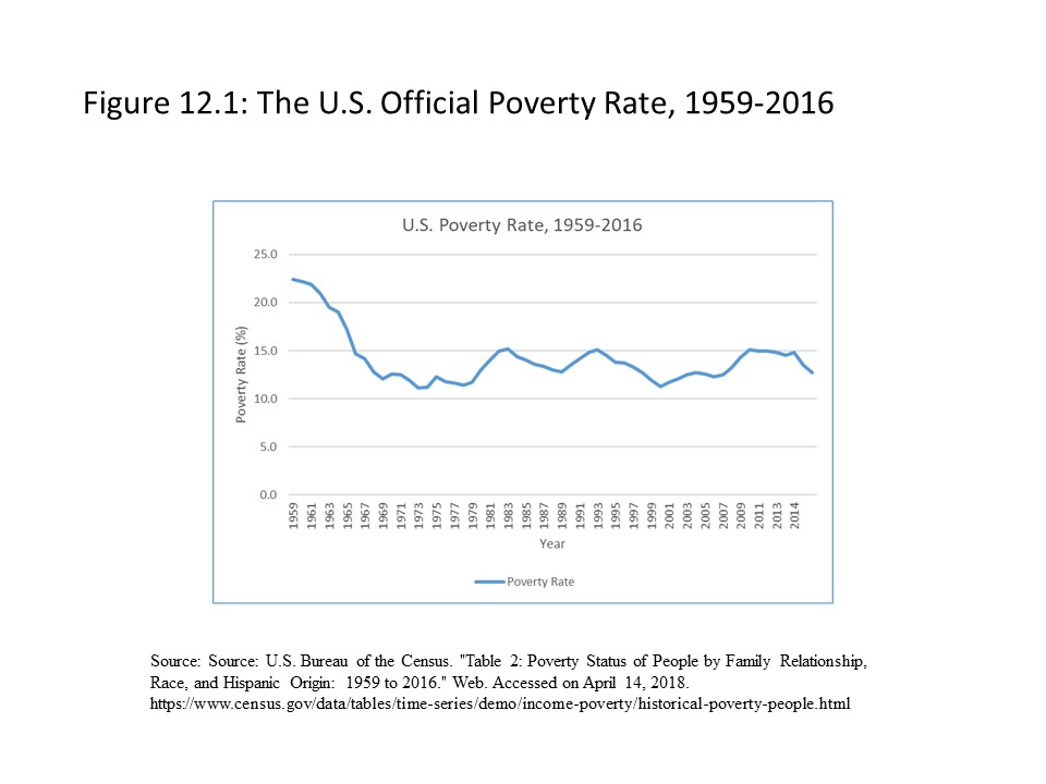 As Figure 12.1 shows, the U.S. poverty rate fell significantly during the economic expansion of the 1960s but rose during the recessions in the early 1980s and early 1990s. It also declined during the economic expansion of the 1990s but rose again after the 2001 recession and even more during the Great Recession. The poverty rate thus seems to follow a somewhat countercyclical movement, which means that it rises during recessions and falls during expansions.
 Table 12.1 arranges the countries from the least equal to the most equal as reflected in the falling quintile ratios as you move down the column. In Table 12.1, Colombia has the highest degree of income inequality, and Norway has the least income inequality of the countries in the table.
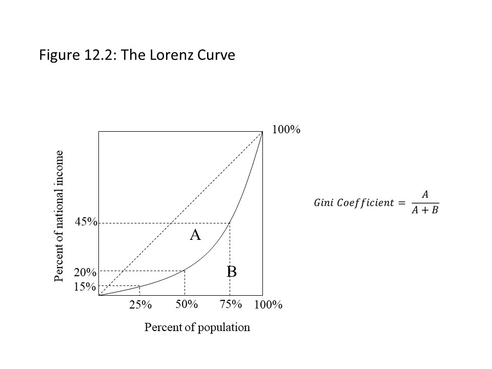
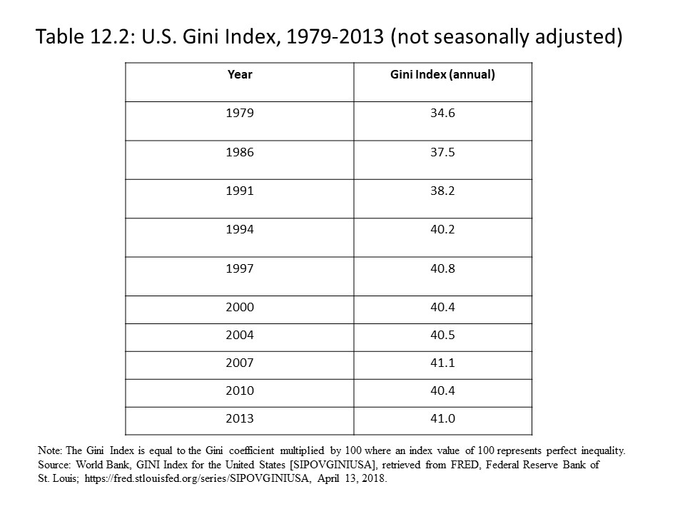 Table 12.2 shows clearly that the level of income inequality in the U.S. has worsened over time. It is also possible to create a Lorenz Curve to represent the distribution of wealth and a Gini Coefficient to measure the extent of wealth inequality. In the U.S., the distribution of wealth has been much more unequal than the distribution of income. Figure 12.3 places Lorenz Curves representing the distribution of income and the distribution of wealth on the same graph.
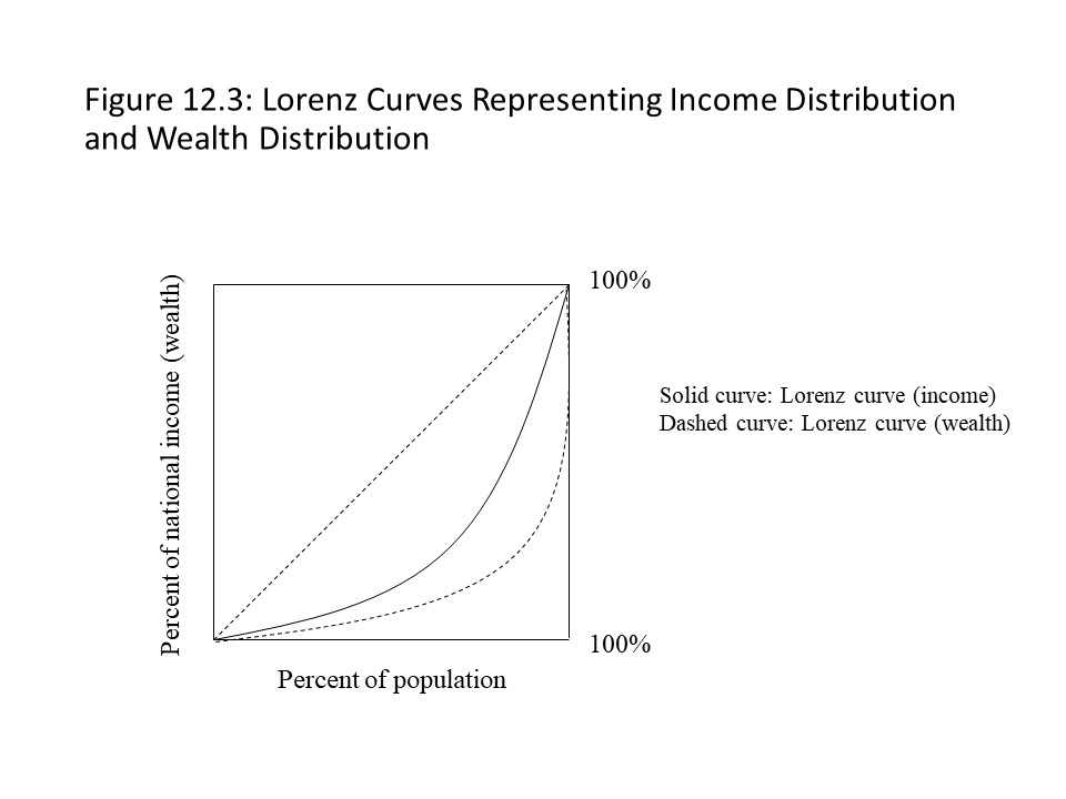
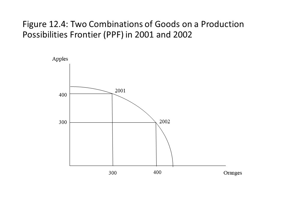 Figure 12.4 shows two combinations of apples and oranges that the economy produces in two different years. In 2001, it produces 400 apples and 300 oranges. In 2002, it produces 300 apples and 400 oranges. The reader should recall that the quantities of each good are measured in real terms (i.e., so many apples and so many oranges). It is not meaningful to add up all the apples and oranges in a year because they are qualitatively different goods. Even if we are satisfied adding together different types of fruit, if the goods produced in this economy included apples and automobiles, then adding these goods together would really make no sense. In general, the fact that differences exist among the units in which each good is measured prevents us from adding together the real quantities.
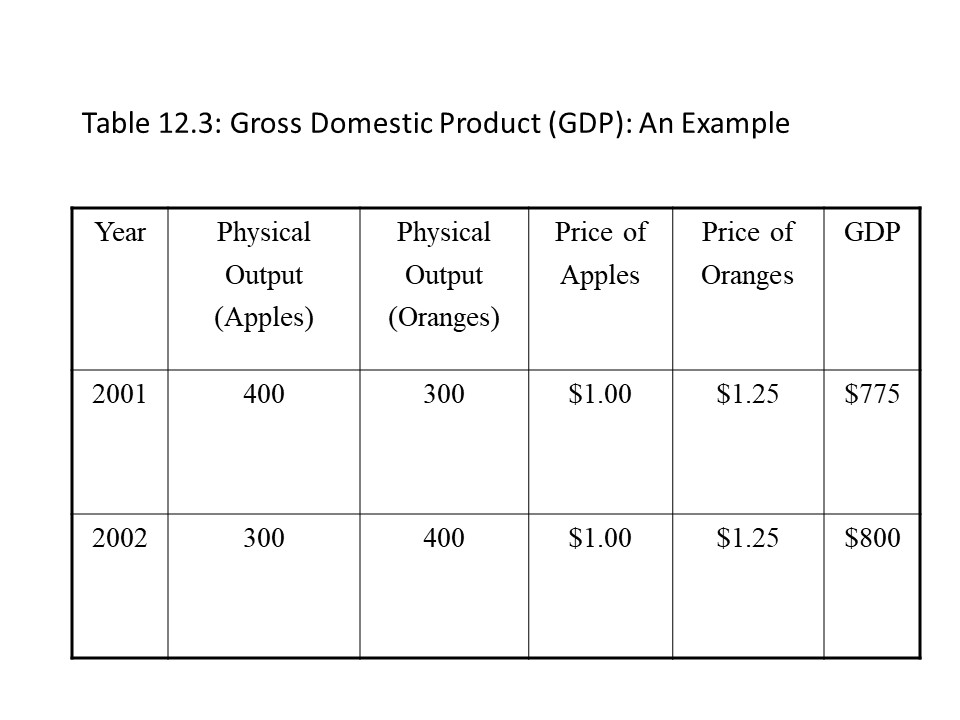 If we multiply each real quantity of a good by the market price of the good, then we obtain a dollar value of that good for the year. We then add the dollar values of apples and oranges for that year and we obtain the aggregate output or GDP for this simple economy. This measure of aggregate output makes it possible for us to compare the size of the economic pie across two years. Since GDP has risen from $775 to $800, we conclude that GDP has risen from 2001 to 2002. Without the common metric that money provides, it would not be possible to draw any conclusions about the change in aggregate output between 2001 and 2002.
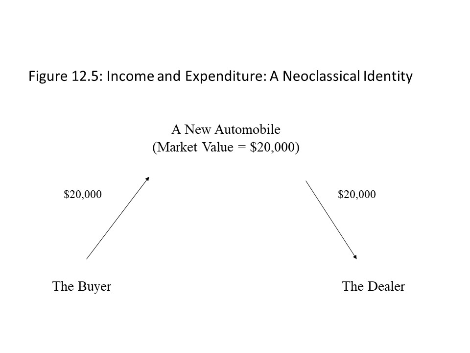 If I purchase that new 2014 Ford Escape for $20,000 in 2014, then we can think about my expenditure of $20,000, which is equal to the value of that final good. We can also think about it from the perspective of the dealer who receives an income of $20,000 when she sells the automobile. At a macroeconomic level, whether we add up all the expenditures on final goods or whether we add up all the incomes received from the sale of final goods, we should obtain the same measure of aggregate output. This result must hold true because of the income-expenditure identity.
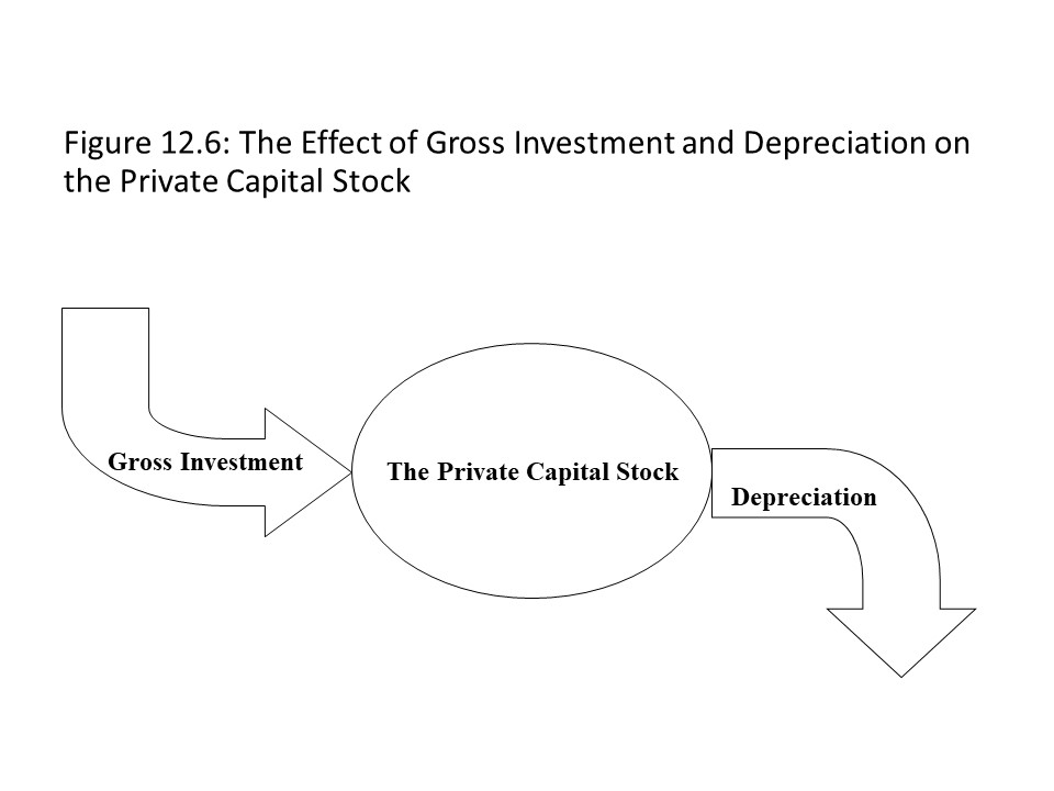 Since gross investment and depreciation cause annual changes in the size of the private capital stock, they are flow variables. The private capital stock is obviously a stock variable because it is measured as of a point in time. If gross investment exceeds depreciation, then the private capital stock expands. That is, more is added to the private capital stock than is depleted. If gross investment is below depreciation, then the private capital stock contracts. That is, more of the private capital stock is wearing out than is being replaced. If gross investment and depreciation are equal, then the private capital stock remains constant for that year.
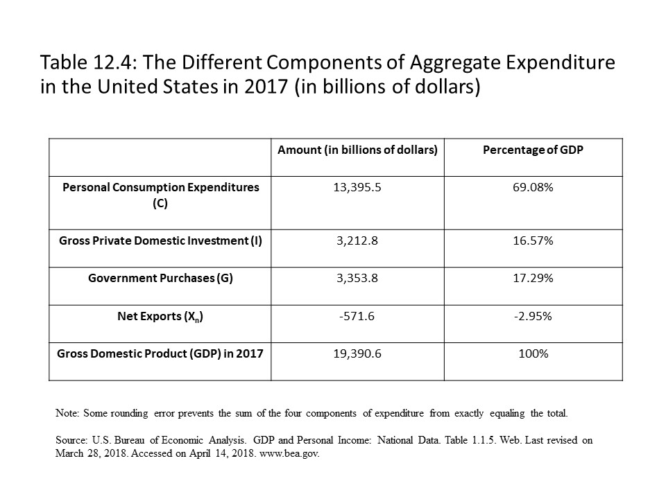 The sum of personal consumption expenditures, gross private domestic investment, government purchases, and net exports is equal to GDP for that year. As Table 12.4 shows, GDP for 2017 was equal to $19.3906 trillion. In general, personal consumption expenditures tend to be about 2/3 (or about 66.67%) of GDP. This statistic is a frequently quoted statistic in the economic news of the nation. It is often stated that consumer spending makes up 2/3 of the economy. When people make this claim, they have in mind 2/3 of GDP. Government purchases are usually about 20% of GDP. Investment spending is typically about 10-15% of GDP. Net exports tend to be the smallest component of aggregate spending at about 3% and have been negative in recent decades. The percentages shown in Table 12.4 are approximately at these levels. Also, the reader should notice that the U.S. trade deficit is reflected in the negative value of net exports.


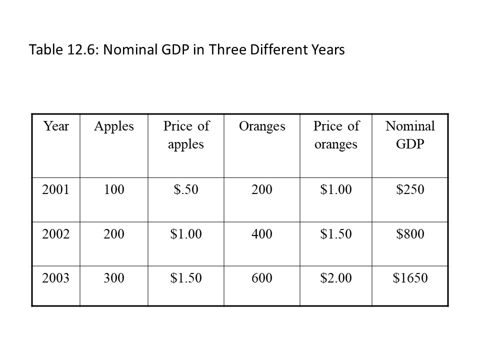 Nominal GDP is calculated by multiplying prices and quantities and summing them up as explained previously. Nominal GDP refers to GDP measured in current year market prices and is the measure that we have been discussing all along. As Table 12.6 shows, nominal GDP rose between 2001 and 2003, but it rose for two reasons. One reason is the increase in real quantities of apples and oranges produced. The second reason is the rise in the prices of apples and oranges. If we want our measure of aggregate output to only capture increases in real quantities produced, then we have a problem. The problem is the result of changing prices and so the obvious solution is to fix the prices. Which prices should we use? We have market prices from three different years that we can use in our calculation. It really does not matter which set of prices we use if they are constant. Because the choice is arbitrary, we will designate one year as the base year and then use the base year prices to calculate GDP for any year.
 That is, 2001 has been selected as the base year and has been used to calculate real GDP. Real Gross Domestic Product (GDP) is the measure of aggregate output using current year quantities and base year or constant prices. It should be clear that Real GDP has risen between 2001 and 2003 but the increase is much less dramatic than the increase in nominal GDP during those years. The reason, of course, is that real GDP only increases because of the increase in real quantities. Nominal GDP, on the other hand, rises due to the increase in real quantities and the rise in market prices. Because Real GDP allows us to focus on changes in real production, it is argued to be a superior measure of aggregate output.
 Reductions in real GDP are considered recessions and increases in real GDP are considered expansions. When real GDP reaches a local maximum, it is considered the peak of the business cycle. When real GDP reaches a local minimum, it is considered the trough of the business cycle. As a rule of thumb, economists usually regard two consecutive quarters of negative real GDP growth as a recession. Recessions vary a great deal, however, in terms of their length and intensity. They can be long and deep or short and mild. The length and intensity of expansions is also difficult to predict.
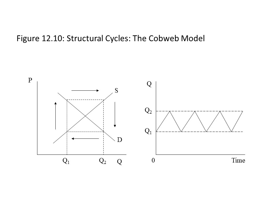 This simple model is referred to as the cobweb model.[19] More sophisticated versions of the cobweb model show the market price gradually approaching the equilibrium price as the adjustments become smaller and begin to approach their target. Assuming many or all individual markets experience such fluctuations, an aggregation of these output fluctuations will produce macroeconomic fluctuations with corresponding fluctuations in employment. Because the explanation of business fluctuations stemming from the cobweb model is rooted in errors made by producers, it may be considered a heterodox theory of economic cycles. As we will see, however, most orthodox and heterodox explanations of business cycles emphasize other factors. Later chapters delve into the sources of these different explanations.
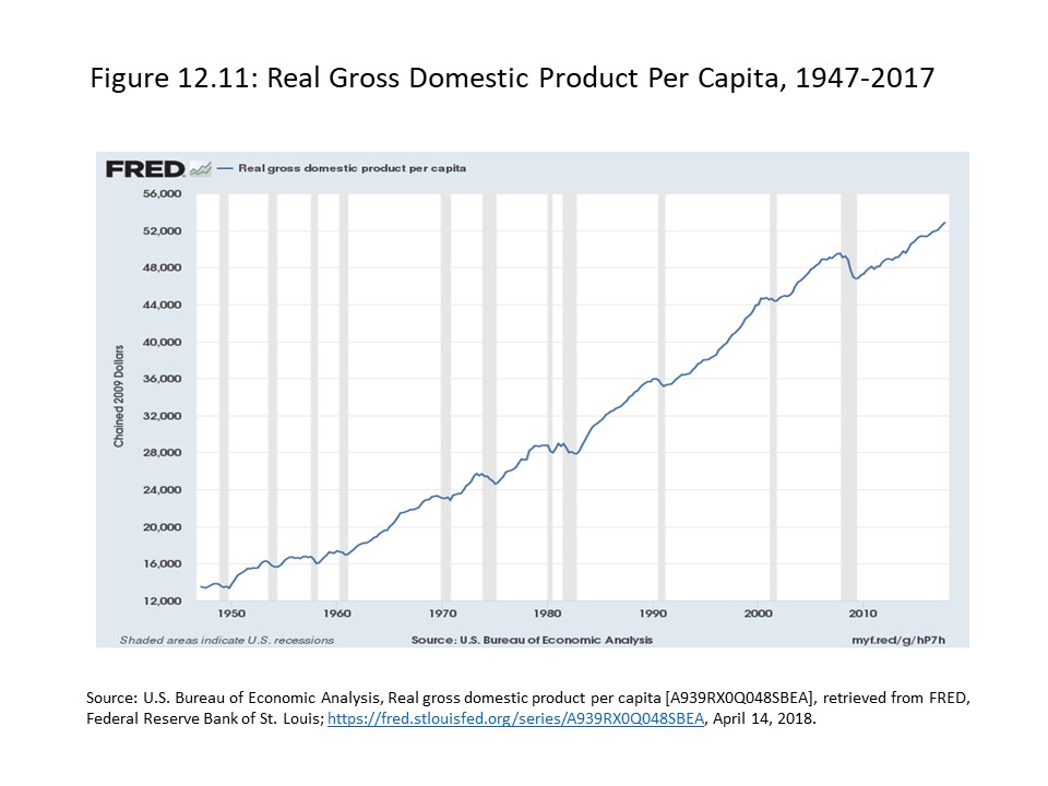 A similar measure that uses real GDP in its calculation is real GDP per worker, which measures the average labor productivity for each member of the labor force as follows.
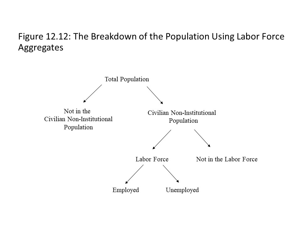 Figure 12.12 shows that the total population may be divided into the civilian non-institutional population and those not in the civilian non-institutional population. Those in the civilian non-institutionalpopulation are at least 16 years old and are not in institutions such as mental hospitals or prisons. Those not in the civilian non-institutionalpopulation are under 16 years of age or are living in institutions. The civilian non-institutional population then may be divided into those in the labor force and those not in the labor force. Those in the labor force are non-institutionalized civilian workers who are willing and able to work. Those not in the labor force are non-institutionalized civilian workers who are not willing or are not able to work. For example, full-time students, retirees, stay-at-home parents, and disabled people are considered not in the labor force. They are of working age but are not willing or able to work at the current time. Of those willing and able to work, those with jobs are considered employed. Those without jobs who have tried to find work within the past four weeks are considered unemployed. If workers have become discouraged and have given up looking for work, then they are considered outside the labor force. Discouraged workers are thus not in the labor force. The four-week cutoff is completely arbitrary and shows how social values creep into the construction of macroeconomic variables like unemployment. That is, some people find this cutoff to be too short when counting people as unemployed. These people wish to count more people as unemployed. Other people find this cutoff to be too long when counting people as unemployed. These people wish to count fewer people as unemployed. The normative content of the unemployment measure was discussed in detail in Chapter 1.
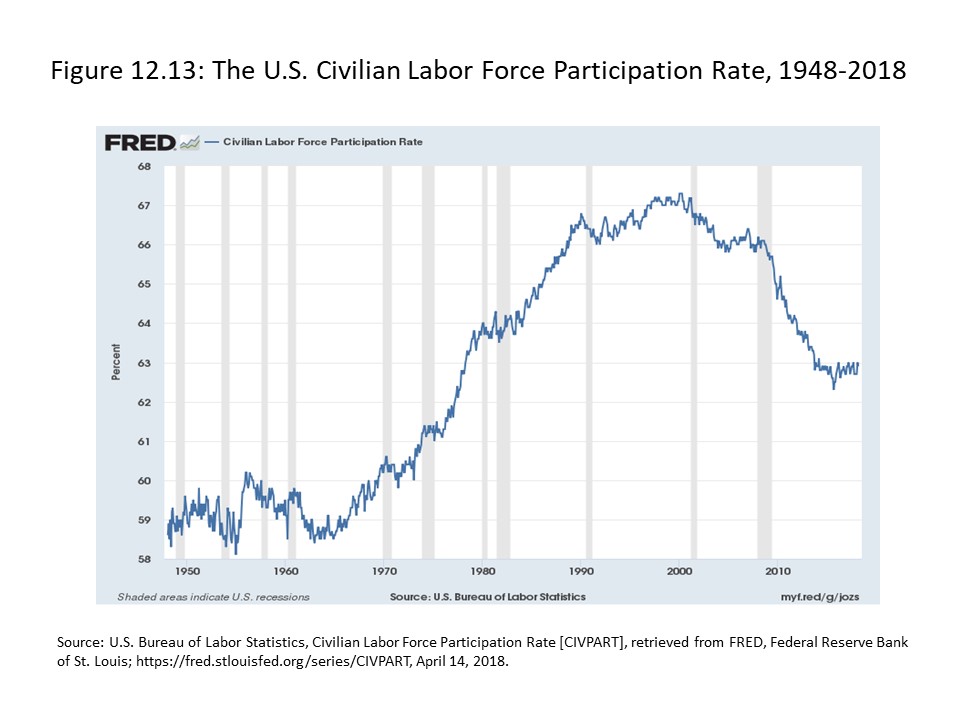 Figure 12.13 shows that the labor force participation rate in the U.S. rose considerably from the 1960s to the 1990s but that it has declined quite significantly since the turn of the century.
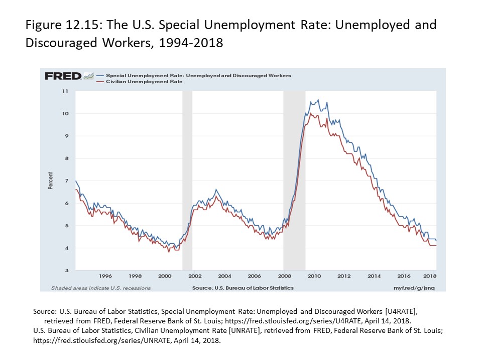

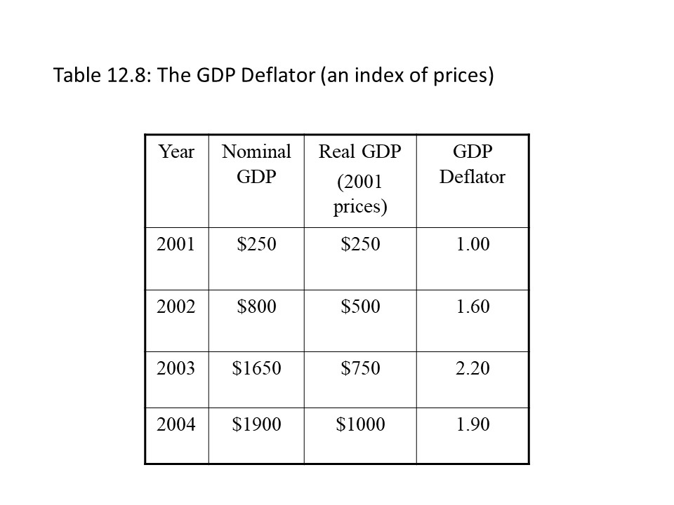
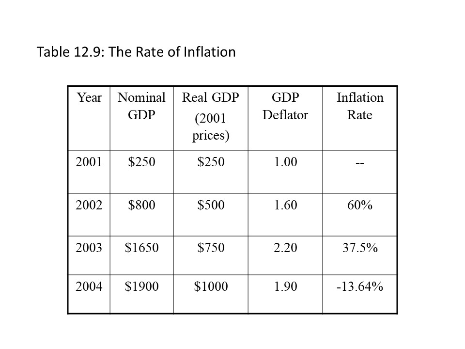


 The base year in this example is 1982-1984. Actual CPI data were used for these calculations and so this decline in the real value of the $1000 is not hypothetical but actual. As Figure 12.18 shows, the real value of the $1000 in 2002 was equivalent to about $550 in 1982-1984 dollars. Therefore, it lost nearly half its value (i.e., its purchasing power). For this reason, people generally try to protect themselves from inflation. People who receive fixed incomes or people who put money under mattresses generally are harmed by inflation. It explains why workers organize themselves into unions to pressure employers for higher money wages and why Social Security recipients are protected with automatic cost of living adjustments to their benefit amounts.
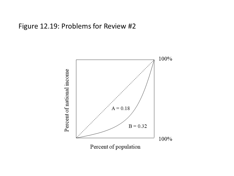 Calculate the Gini coefficient. If the Lorenz curve then shifts and becomes closer to the diagonal line, what should happen to the Gini coefficient and what would you conclude about the degree of income inequality in this country?
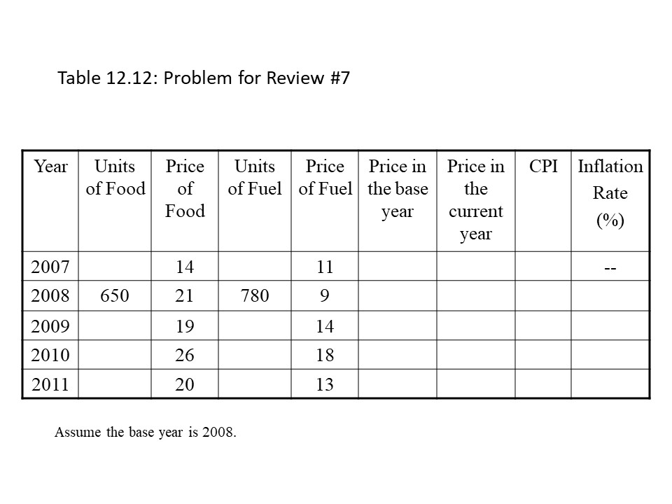 8. If your nominal income is $2,000 per month in 2018 and the CPI is 1.40 with 2011 as the base year, then what is the real value of your monthly income in constant 2011 dollars?