Define Say’s Law of Markets and its role in classical economic theory
Describe how John Maynard Keynes created a revolution in macroeconomic theory
Analyze the Keynesian Cross model and the Keynesian multiplier effect
Build the aggregate demand/aggregate supply (AD/AS) model to explain the price level and level of aggregate output
Apply the AD/AS model to several historical cases from U.S. economic history
Identify the Neoclassical Synthesis Model and the Post-Keynesian critique of it
This chapter introduces the reader to macroeconomic theory. One major goal is to describe how the key macroeconomic variables from the previous chapter are determined using theoretical models. To really understand these theoretical models, however, it is helpful to explain how the field of macroeconomics developed in the first place. This chapter thus explains the way in which John Maynard Keynes led a revolution in economic thought in the 1930s. Keynes laid the groundwork for what became known as macroeconomics. To understand Keynes’s role in the history of economic thought, it is necessary to understand his critique of the classical theory of the aggregate economy and one of its key elements known as Say’s Law of Markets. Once Keynes’s role is made clear, it will be easier to understand his theory of output and employment. This theory is represented in the Keynesian Cross model and Keynes’s concept of the spending multiplier. We will also build the aggregate demand/aggregate supply (AD/AS) model so as to provide an explanation, not only for aggregate output and employment, but also for the general level of prices. Using the AD/AS model, we will use it to understand actual changes in aggregate output and the price level that occurred during different periods in U.S. economic history.
Say’s Law and the Classical Theory
It might strike the reader as strange that economics is divided into two separate fields referred to separately as “microeconomics” and “macroeconomics.” This division has not always existed. During the eighteenth and early nineteenth centuries, the discipline was simply referred to as “political economy.” Economists generally regarded questions at the individual level and questions at the societal level as questions to be treated together. During the marginalist revolution of the late nineteenth century, however, some economists became very much preoccupied with questions of efficiency and individual optimization. Larger questions having to do with economic growth, the general level of prices, and overall employment became increasingly separate from this specialized study of atomistic behavior. In 1936, this bifurcation intensified when John Maynard Keynes published his famous book titled, The General Theory of Employment, Interest, and Money. Published shortly after the Great Depression, Keynes offered a theory to explain how aggregate output, employment, and prices are determined. His explanation sharply contrasted with early neoclassical microeconomic theories of how individual markets function.
In his critique of early neoclassical microeconomic theory, Keynes referred to the theory as the “classical” theory. Keynes’s decision to do so stemmed in part from the fact that early neoclassical theory had a laissez-faire orientation that was very similar to the laissez-faire orientation of the classical theories of Adam Smith and David Ricardo. His decision also stemmed from his critique of one aspect of classical economics that was central to early neoclassical thinking, referred to as Say’s Law of Markets. According to Say’s Law of Markets (or Say’s Law, for short), every supply creates its own demand. That is, if a commodity is produced, it will generate enough factor income for the owners of land, labor, and capital to purchase the produced commodity. After all, the price of the commodity may be divided into its component parts of rent, wages, and profits. Hence, these incomes will be sufficient to realize the price of the commodity. The stunning implication of this simple argument at the level of the aggregate economy is that enough income will always exist to purchase the entire output of commodities. Therefore, no general gluts or periods of overproduction are possible. Using nothing but logic, one can conclude that major depressions should never occur. If they do occur, they must be caused by some interference with the free flow of commodities and money, and government interference is a likely culprit. Say’s Law thus supported the laissez-faire orientation of classical economics and early neoclassical economics later.
Another way to understand the classical theory of output and employment is to consider the way in which competition in the labor market will lead to a full employment equilibrium outcome, as depicted in Figure 13.1.[1]
If the market wage (w) is above the equilibrium wage (w*), then a surplus of labor or unemployment exists. Competition will force the market wage down until the market wage coincides with the equilibrium wage. The surplus will be eliminated and the quantity of labor demanded will equal the available labor force (Lf*). With the economy operating at full employment, the economy will be able to produce at the full employment level of GDP (GDPf*). The full employment GDP is shown in Figure 13.1 using the aggregate production function. The aggregate production function exhibits diminishing returns to labor, which assumes that all other factors of production (e.g., land and capital) are held constant. Of course, all available land and capital will be fully employed as well, assuming that the markets for these resources have cleared as well. Given the available production technology and the fully employed resources, the economy will produce the potential GDP.
John Maynard Keynes’s General Theory of Employment, Interest, and Money
John Maynard Keynes was well-trained in neoclassical economic theory. In fact, Keynes’s critique of neoclassical theory was not intended to undermine it entirely. Instead, Keynes regarded that theory as applicable to a special case only, namely the case of an economy operating at full employment. That is, once the economy operates at full employment, then all of the efficiency conclusions of neoclassical theory apply once again. Keynes’s theory was intended to be a more general theory of how the aggregate economy functions, however, and so it offered a framework for thinking about periods during which the economy failed to achieve full employment. To make this argument, Keynes had to attack that central tenet of classical economic theory known as Say’s Law. The simple flow diagram in Figure 13.2 helps to illustrate Keynes’s argument.[2]
As Figure 13.2 shows, business enterprises make payments to households in exchange for the resources households sell to businesses. Households receive factor income for the land, labor, and rent that businesses purchase. The businesses use these factors of production to produce finished commodities. The households then spend this factor income on the finished commodities, but it is here that we deviate from our earlier discussion of the neoclassical circular flow model from Chapter 3. Obviously, households will choose to save some of their income and not spend it. The classical economists and early neoclassical economists understood this point well. They argued that the saving that occurred would flow into the loanable funds market where it would be transferred to individuals and firms who would invest it. These investments in new capital goods would add to the demand for consumer goods and ensure that all of the finished commodities were sold. Of course, these borrowers would pay interest to the lenders for the use of the borrowed funds, but the circular flow would be maintained and Say’s Law would hold.Figure 13.3.
If a surplus of savings exists, then in the classical theory, the market rate of interest (i) will fall to the equilibrium level of i* and clear the loanable funds market. Aggregate saving will equal aggregate investment. If, however, other forces are acting on the rate of interest that prevent it from falling, then the surplus of savings will persist and not all savings will be invested. As a result, not all finished commodities will be sold due to insufficient investment demand. Alternatively, it might be that the market clearing level of the rate of interest (i*) does not occur at a market rate of interest that is greater than or equal to zero due to a very large supply of savings and a relatively low level of investment demand. In that case, the market rate of interest will not be able to fall enough to clear the market for loanable funds and the surplus of savings will persist. In this case as well, an excess supply of finished commodities or a glut will occur. The result will be falling production as firms scale back production, falling employment as they lay off workers, and falling prices due to the excess supplies of commodities. All these results were observed during the Great Depression, which is exactly what Keynes developed his theory of effective demand to explain with the hope of ending depressions by means of enlightened government economic policy.
The Consumption Function and the Saving Function
To understand the theory that Keynes developed, it is necessary to begin with the construction of some foundational elements. We first introduce the consumption function and show how it is represented graphically. The consumption function suggests that a positive relationship exists between the level of current consumption expenditures that households are planning and the current level of disposable income. That is, as households acquire more disposable income, their level of consumption rises, other factors held constant (ceteris paribus). Planned consumption thus depends on the disposable income of households. That is, C is a function of DI or C = f (DI). Alternatively, C is the dependent variable and DI is the independent variable, according to this theory. This relationship can be represented mathematically as follows:
In the consumption function, CO represents autonomous consumption. Autonomous consumption is the level of consumption expenditures that households choose even if their DI falls to zero (i.e., an amount that is independent of income). Such expenditures might be possible if households rely on their savings to finance consumer expenditures. Borrowing would be another way in which consumer expenditures might be positive even when DI equals zero. The consumption function also includes ΔC/ΔDI, which represents the marginal propensity to consume (mpc). The mpc refers to the additional consumption expenditures that households choose for each additional dollar of disposable income received. Figure 13.4 reveals that the level of autonomous consumption determines the vertical intercept of the consumption function in the graph. Similarly, the mpc represents the slope of the consumption function in the graph.
Because the mpc is assumed to be fixed at every level of DI, the slope is constant and the consumption curve graphs as a straight line. To consider a simple example, suppose that the consumption function is C = 200+0.75DI. In this case, even if DI is equal to zero, the households will spend $200 billion. Also, for every $1 of additional DI that the households receive, they will consume an additional $0.75.
It is worth noting that only a change in DI can cause a movement along the consumption curve in the graph whereas a change in autonomous consumption will shift the consumption curve up or down. Various factors can shift the consumption curve up or down. One example is a change in household wealth, which is distinct from disposable income. The reader might recall that DI is a flow variable. That is, it is measured per period of time (e.g., per year). Household wealth, on the other hand, is a stock variable and is measured at a point in time. If households experience a reduction in household wealth due to a recession that causes asset values (e.g., stock prices) to fall, then the consumption expenditures will fall at every level of disposable income and the consumption curve will shift in a downward direction. Alternatively, an economic boom that raises household wealth will cause the consumption curve to rise at every income level and will lead to an upward shift.
Just like we can represent the level of planned household consumption expenditures, we can also represent the level of planned household saving as the level of disposable income changes. The saving function suggests that a positive relationship exists between planned household saving and disposable income. That is, as households acquire more disposable income, their level of saving rises, other factors held constant (ceteris paribus). Planned saving thus depends on the disposable income of households. That is, S is a function of DI or S = f (DI). Alternatively, S is the dependent variable and DI is the independent variable, according to this theory. This relationship can be represented mathematically as follows:
In the saving function, SO represents autonomous saving. Autonomous saving is the level of saving that households choose even if their DI falls to zero (i.e., an amount that is independent of income). Such “saving” might occur if saving is negative. That is, households do not save but actually borrow or draw down past savings. The saving function also includes ΔS/ΔDI, which represents the marginal propensity to save (mps). The mps refers to the additional saving that households choose for each additional dollar of disposable income received. Figure 13.5 reveals that the level of autonomous saving determines the vertical intercept of the saving function in the graph. Similarly, the mps represents the slope of the saving function in the graph.
Because the mps is assumed to be fixed at every level of DI, the slope is constant and the saving curve graphs as a straight line. To consider a simple example, suppose that the saving function is S = -200+0.25DI. In this case, even if DI is equal to zero, the households will save -$200 billion. Also, for every $1 of additional DI that the households receive, they will save an additional $0.25.
It is worth noting that only a change in DI can cause a movement along the saving curve in the graph whereas a change in autonomous saving will shift the saving curve up or down. Various factors can shift the saving curve up or down. A rise in household wealth will lead to a fall in saving (as consumption rises) and shift the saving curve downward. A fall in household wealth will lead to a rise in saving and shift the saving curve upward. As in the case of consumption, planned saving by households represents a flow variable.
It is worth taking a moment to reflect on the relationship between the vertical intercepts of the consumption and saving functions. In both cases, the level of DI = 0, which implies that C+S = 0. This equation further implies that when DI = 0, C = -S. In other words, the vertical intercept of the saving curve is the negative of the vertical intercept of the consumption curve. Therefore, whenever the consumption curve shifts upward, the saving curve will shift downwards, and vice versa. Figure 13.6 shows how a shift of the consumption curve will lead to an opposite change in the saving curve.
One should also consider the relationship between the mpc and the mps. Suppose we add the two measures together as follows:
In other words, the sum of the mpc and the mps is always equal to 1. This result is very intuitive. If the households receive $1 of additional DI and they consume $0.75 of it, then the remaining $0.25 must be saved.
Now that we understand the essential building blocks of Keynes’s theory, we need to consider a national income accounts identity that relates disposable income (DI) to consumption (C) and saving (S).
We then consider the case in which S = 0 and thus C = DI. To represent this case graphically, we introduce a reference line that has a 45 degree angle relative to the horizontal axis as shown in Figure 13.7.
As Figure 13.7 indicates, at each level of DI, the level of C that corresponds to it is found on the reference line. That is, the horizontal distance to that level of DI will be exactly the same as the vertical distance from that level of DI up to the 45 degree line. Another way to think about this reference line is that it has a slope equal to 1 and a vertical intercept equal to zero, much like the equation y = x in the case that y is placed on the vertical axis and x is placed on the horizontal axis.Figure 13.8, however, we see that the difference between the two lines carries a special meaning.As Figure 13.8 shows, at a level of DI of $1000 billion, the reference line allows us to represent that amount vertically. It is then much easier to see which part of the DI is spent on consumption and which part remains for saving. In this case, $800 billion is consumed and $200 billion is saved. In general, at every level of DI at which the C line is below the reference line, positive saving exists. The reader will notice that the lines intersect at a single point. At this point, planned consumer spending equals DI, which is true for all points on the reference line. When planned consumer spending equals DI, we refer to this income level as the break-even income level. In other words, households have just enough DI to finance their consumption expenditures, no more and no less. Finally, if DI is at a low enough level that the C line is above the reference line, then planned household consumption expenditures exceed DI and the households must be borrowing or relying on past savings to finance the excess consumption.Figure 13.9 depicts the relationship between the two graphs.
At the break-even income level of $40 billion in the top graph, C = DI and thus S = 0. Therefore, the bottom graph shows the saving function crossing the DI axis at $40 billion, indicating a level of saving equal to zero at that level of DI. As we move to the right of the break-even income level in the top graph, we see that saving becomes positive and continues to grow as the gap between the two lines becomes larger. Therefore, in the bottom graph, the level of saving becomes positive and continues to grow when DI rises above $40 billion.
Let’s suppose we are given the following consumption function:
It turns out that it is possible to derive the saving function from this information. Recall that DI = C+S. Substituting the consumption function into this equation yields DI = 20+0.75DI+S. Solving for S yields S = DI – 0.75DI – 20, which may be simplified as follows:
It should be clear that we can use a shortcut method to obtain the saving function from the consumption function. If we begin with the consumption function and negate the vertical intercept of 20, then we obtain the vertical intercept of -20 for the saving function. Furthermore, if we subtract the mpc of 0.75 from 1, then we obtain the mps of 0.25 since the two marginal propensities always add up to 1.
The Keynesian Cross Modelfor a Private, Closed Economy
It should be clear that Keynes radically departed from the early neoclassical economic theory in which he was trained. In Keynes’s theory, aggregates, like households, business enterprises, and the government, take center stage. Individual economic agents do not play an important role in the theory. Also, because households and businesses tend to behave in a collective fashion (e.g., consuming more when DI rises or investing less when business expectations turn sour), mass psychology becomes the primary explanation for these behaviors rather than individual rationality and serves as an alternative conceptual point of entry.[4] For example, households have a propensity to consume so much more when DI rises. Nevertheless, the unidirectional logic of neoclassical theory is preserved in Keynes’s theory.[5] That is, one variable affects another in a single causal direction only. For example, a rise in DI causes a rise in consumer spending, but not vice versa.
Based on this theoretical foundation, it is now possible to develop the basic Keynesian theory of output and employment. The Keynesian Cross model, which is also sometimes referred to as the aggregate expenditures model, uses these theoretical tools to explain the equilibrium levels of aggregate output and employment that emerge. To keep the model simple, we initially assume that the economy is private and closed. That is, only households and businesses exist. Because it is a purely private economy, no government exists. Because it is a closed economy, no foreign trade exists. The price level is also assumed to be constant and so the Keynesian Cross model does not explain prices, only output and employment. Finally, it is assumed that DI is equal to real GDP. In the national income accounts, the income that American households have for consumption and saving (DI) is not equal to real GDP due to the presence of depreciation, net foreign factor income, taxes, and transfer payments. With a closed, private economy without depreciation, no such adjustments need to be made, and DI is equal to real GDP.
To build the Keynesian Cross model, we need to explain the determination of planned investment spending. As explained previously, the level of planned investment spending is determined in the loanable funds market. Savers lend funds to borrowers at interest, and their competitive interaction determines a particular quantity of loanable funds exchanged. These loanable funds are invested in new production plants and equipment. If we assume that the level of planned investment spending is independent of the level of real GDP, then we can represent its determination in the loanable funds market as shown in Figure 13.10 below.
As the reader can see in the graph on the right, investment spending (I) is equal to IO and is thus constant at all levels of real GDP (Y).
It is now possible to write two equations representing the two types of planned expenditures in this simple economy. The consumption function representing the planned consumption of households may be written as:
The reader should notice that real GDP (Y) has replaced DI in the consumption function. The reason, of course, is the assumption that real GDP is equal to DI in this economy. The second equation indicates that investment spending (I) is constant, as previously noted.
If we combine these two types of planned spending, we can obtain a planned aggregate expenditures (A) function as follows:
This planned aggregate expenditures function may be written as follows by rearranging the terms:
In this function, CO + IO represents autonomous spending. That is, households and businesses will select this level of planned spending regardless of the level of real GDP. The second portion, (ΔC/ΔY)Y, represents induced spending. Induced spending is planned aggregate spending that is directly related to the level of real GDP. If we place the planned consumer spending (C) curve and the planned aggregate expenditures (A) curve on the same graph, we obtain the graph shown in Figure 13.11.
As the reader can see, the planned aggregate expenditures curve has a vertical intercept equal to the level of autonomous spending. The vertical distance between A and C is constant and equal to IO at every level of DI. The slope of the aggregate expenditures curve is also equal to the mpc because the A and C curves are parallel to one another.Figure 13.12 shows that the equilibrium level of real GDP occurs at the intersection of the aggregate expenditures curve and the 45-degree reference line.
At this point, planned aggregate spending equals real aggregate output and so all plans are perfectly satisfied by the level of production. The reason this level of real GDP is the equilibrium level can be understood by considering what will occur if the economy is not producing at this point. Suppose that the level of real output is above Y* in the graph. In that case, planned aggregate spending is below the level of real output as shown on the 45-degree line. That is, A < Y. As a result, firms will be producing more than households and firms wish to purchase. As a result, business inventories will build up as a result of the excess supply of commodities. The consequence will be a drop in the level of production as firms cut production. Real GDP will then fall towards the equilibrium level. Conversely, if the level of real GDP is below Y* in the graph, then planned aggregate spending is above the level of real output as show on the 45-degree line. That is, A > Y. As a result, firms will be producing less than households and firms wish to purchase. As a result, business inventories will be depleted as a result of the excess demand for commodities. The consequence will be a rise in the level of production as firms raise production. Real GDP will then rise towards the equilibrium level.
It is also possible to calculate the equilibrium real GDP given a specific consumption function and level of investment. For example, suppose that the following two equations represent an economy:
Given this information, it is possible to obtain the planned aggregate expenditures function by simply adding the two equations together:
To obtain the equilibrium real GDP for this economy, we need to use the equilibrium condition:
Plugging in the planned aggregate expenditures function and solving for Y, we obtain the equilibrium level of real GDP.
Figure 13.13 represents the solution graphically.
The graph shows that the equilibrium level of real GDP occurs at the intersection of the reference line and the planned aggregate expenditures curve. Solving the two equations simultaneously yields the solution.
It turns out that it is possible to think about the determination of the equilibrium real GDP from another angle. That is, by using the saving function and considering the level of investment spending, it is possible to arrive at a different but related equilibrium condition. To understand this point, consider the equilibrium condition that we have been using up to this point:
The reader should recall that planned aggregate spending (A) is the sum of planned consumer spending (C) and planned investment spending (I). Real GDP or real income (Y) is either consumed (C) or saved (S). If we break down each term in the equation into its component parts, we obtain the following:
It is easy to see that the level of consumer spending may be subtracted from both sides of this equation to yield a new equilibrium condition:
In equilibrium then, planned investment and saving must be equal. Figure 13.14 represents this solution graphically and relates it to the Keynesian Cross model that we have already discussed.
Because planned investment is constant at all levels of GDP, it is represented as a horizontal line in the graph. The saving curve, on the other hand, slopes upward for reasons already discussed. The equilibrium level of real GDP occurs at the intersection of the two lines.Figure 13.15.
In Figure 13.14, if the level of real GDP is below the equilibrium level of Y*, then planned investment exceeds saving. With the injection larger than the leakage, the result is a rise in real GDP and a movement towards the equilibrium level. On the other hand, if the level of real GDP is above the equilibrium level of Y*, then saving exceeds planned investment. With the leakage larger than the injection, the result is a fall in real GDP and a movement towards the equilibrium level.
It is also possible to arrive at the answer algebraically using the same information we used when discussing the Keynesian Cross model. Because we know the shortcut method of deriving the saving function from the consumption function, we can write the saving function alongside the consumption function as follows:
Given that I = 100, we use the new equilibrium condition as follows:
We then solve for Y to obtain:
The reader will note that this equilibrium real GDP is the same as the one calculated in the Keynesian Cross model. Figure 13.16 shows the solution in a saving-investment graph.
The reader might be a bit confused by the claim that saving equals investment only in equilibrium. After all, it was argued in Chapter 12 that GDP is always equal to the sum of consumer spending, investment spending, government spending, and net export spending. In a closed, private economy without government spending or net exports, GDP should always equal consumer spending plus investment spending. Therefore, if GDP is the sum of consumer spending and saving, then saving should always equal investment spending. The reason for the apparent contradiction is that the equilibrium condition only refers to planned investment whereas the measurement of GDP includes actual investment. In other words, saving will always equal actual investment, which includes both planned investment spending and inventory (unplanned) investment spending. At the same time, saving may not equal planned investment spending. Figure 13.17 clarifies this point.Figure 13.17, if GDP exceeds the equilibrium level of Y*, then saving exceeds planned investment. At the same time, saving is still equal to actual investment because the part of what is saved that is not intentionally invested is unintentionally invested in inventories. That is, not all commodities are sold and so firms will add these commodities to their inventories, which counts as unplanned inventory investment. Therefore, the national income accounts identity holds, but the equilibrium condition, which requires that saving equals planned investment, does not hold.
It is now possible to clearly distinguish the Keynesian model of output and employment from the classical model. Figure 13.18 shows clearly that the level of planned aggregate expenditure determines the equilibrium level of GDP, which is likely to be below the full employment GDP (Yf) at a point in time.
Furthermore, as businesses adjust production in the movement to equilibrium, they also adjust their workforces. Employment, therefore, moves towards an equilibrium level of L* that corresponds to the equilibrium level of real GDP as shown on the production function. Employment also ends up below the full employment level of Lf. Hence, Keynes’s theory is one of unemployment equilibrium, and it reveals the case of full employment GDP to be a special case. That is, aggregate planned spending would need to be just high enough to produce the full employment GDP as the equilibrium GDP. Keynes could, therefore, argue that his theory was a more general theory than the classical theory of employment and output.
The Paradox of Thrift
An interesting application of the model allows us to understand what macroeconomists mean by the paradox of thrift. In Chapter 2 we learned that an increase in saving leads to greater capital accumulation and an expansion of production possibilities. When considering short run macroeconomic fluctuations, however, saving may lead to a very different result. Suppose that all households decide to increase saving at every level of GDP. In other words, autonomous saving rises. When this change occurs, the saving curve shifts upward as shown in Figure 13.19.
Initially, saving rises at Y1, but this increase in saving causes a discrepancy between saving and planned investment spending. Specifically, saving rises above planned investment spending. With the leakage of saving being higher than the injection of planned investment, real GDP begins to fall. The drop in real GDP causes a movement along the new saving curve. In other words, induced saving declines. The reduction in saving continues until it once again equals planned investment and the economy returns to equilibrium at Y2. The problem for the economy is that the high level of saving has led to a recession (i.e., falling real GDP) rather than to economic growth, as suggested by the production possibilities model. Furthermore, and rather paradoxically, even though all households decided to save more, aggregate saving returns to the same level that previously existed.[6] The reason is that the recession has led to falling incomes, which reduces saving.
This example illustrates what neoclassical economists refer to as the fallacy of composition. People often assume that when one person acts in a particular way and achieves it that the same will hold true for groups of people. To use a classic example, an individual attending a sporting event might stand up to obtain a better view of the field. This strategy works, but if everyone has the same idea, then when all stand, no one has a better view than before. Similarly, one household might save more of its income successfully, but if all households do the same, then no one is able to save more.
The Multiplier Effect
Now that the Keynesian Cross model has been developed, we can consider one of Keynes’s most important contributions to our understanding of the manner in which changes in spending affect the overall economy. The Keynesian multiplier effect refers to the way in which an increase in a specific component of spending, such as investment spending, raises real GDP by a multiple of the spending increase. To illustrate this point, we will consider the most volatile component of aggregate spending and the impact of changes in it on real GDP. Investment spending tends to be highly volatile for a number of reasons. It is influenced by business expectations about future profits, interest rates, technological change, and taxes on profit income. Suppose that business expectations about future profitability improve significantly. With businesses feeling more optimistic about the future of the economy, a collective rush to invest in new capital takes place. Keynes referred to such impulses during periods of business optimism as animal spirits. The consequence is a rise in demand in the loanable funds market. Such an increase leads to a rise in the equilibrium level of loanable funds exchanged and to a rise in planned investment spending as shown in Figure 13.20.
The rise in planned investment raises the aggregate expenditures curve as shown in Figure 13.20. The result is a higher level of equilibrium real GDP and the economy experiences an economic boom. Interestingly, the graph on the right in Figure 13.20 suggests that the level of real GDP rises by more than the rise in planned investment. Because the slope of the reference line is equal to 1 and the difference between the old and new A curves is equal to the change in planned investment, the first move up along the reference line would indicate a rise in real GDP equal to the rise in planned investment spending. As the reader can see in the graph, however, real GDP rises by more than this amount. Hence, a multiplier effect is implicit in the Keynesian Cross model.
It is worth asking why this change occurs. Intuitively, when businesses engage in new investment spending, they raise real GDP by the amount of the investment spending. This spending is received as income by the households though. Once received, the households spend a portion of the additional income, which is determined by the marginal propensity to consume. That additional expenditure is received by the households as well, and part of it is spent. This cycle continues indefinitely but the spending that occurs in the successive rounds becomes smaller and smaller due to the saving that occurs in each round. Ultimately, aggregate real GDP rises by a finite amount but also by a multiple of the initial amount of investment spending.
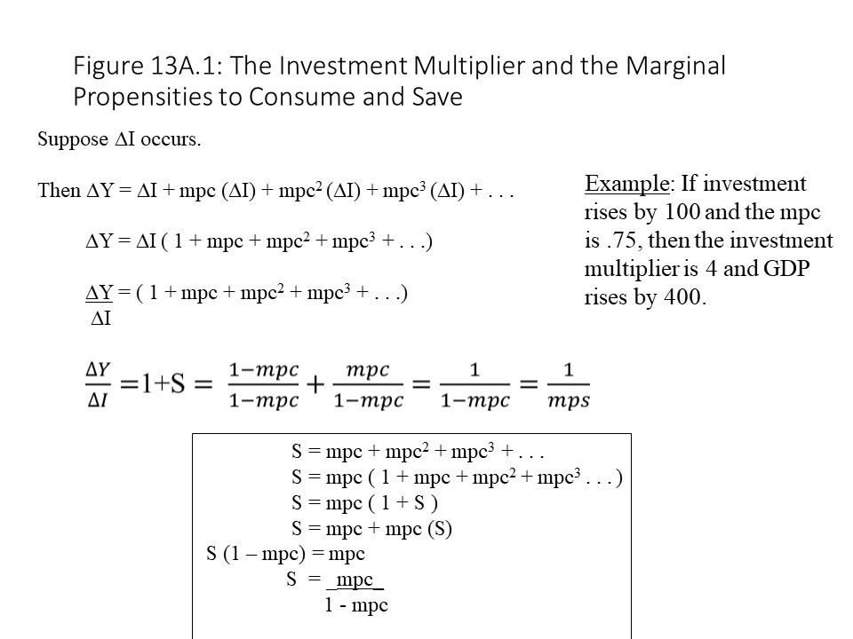
It is possible to derive a formula that tells us the exact impact that a change in investment spending has on real GDP, other factors held constant. Let’s define the investment multiplier as the ratio of the change in real GDP to the change in planned investment spending. By taking into account the way in which the households engage in an infinite series of consumer spending rounds, we can prove that the multiplier is positively related to the marginal propensity to consume as shown below.
Figure 13A.1 provides the details of the proof for any interested readers. Our main purpose, however, is to understand the intuition behind the formula and to learn how to use it to calculate changes in real GDP. To understand how to use the formula, let’s assume that planned investment spending rises by 100. If the mpc is 0.75, then we can calculate the investment multiplier by plugging the mpc into the formula as follows:
Because investment spending rises by 100, we can write the equation as follows:
By solving for the change in GDP, it is clear that real GDP will rise by $400 billion in this case. Alternatively, the multiplier implies that for every $1 of additional investment spending, real GDP will rise by $4.
The Keynesian Cross Model ofan Open, MixedEconomy
In this section, we would like to expand the Keynesian Cross model to include international trade and government activity. To account for these types of expenditure, we will make some simplifying assumptions. First, we will assume that net exports are exogenously given as follows:
In other words, net exports are at the same level regardless of the level of real GDP as shown in Figure 13.21.
As Figure 13.21 shows, net exports may be positive (XnO), equal to zero (Xn1), or negative (Xn2). The reader should recall that net exports equal exports (X) minus imports (M). As explained in Chapter 12, if net exports are positive, then a trade surplus exists (X > M). If net exports are negative, then a trade deficit exists (X < M). If net exports are equal to zero, then balanced trade exists (X = M).Figure 13.22.[7]
In the Keynesian Cross model, we can now add net exports to the consumption function and level of planned investment spending to obtain the aggregate expenditures function as follows:
As the reader can see, autonomous spending now includes net export spending. Otherwise, the aggregate expenditures function is the same. Because net exports may be positive, negative, or equal to zero, the vertical intercept may be above, below, or the same as the aggregate expenditures curve for the closed, private economy. Figure 13.23 shows the case of a trade surplus and the impact that it has on the position of the aggregate expenditures curve relative to that of a closed, private economy.
As the figure shows, the opening of the economy shifts the aggregate expenditures curve upward due to the trade surplus that results.Figure 13.24 shows what happens when the economy runs a trade surplus or a trade deficit.
As Figure 13.24 shows, a trade surplus raises the aggregate expenditures curve and increases the equilibrium real GDP. A trade deficit, on the other hand, lowers the aggregate expenditures curve and reduces the equilibrium real GDP. Balanced trade leaves the aggregate expenditures curve unchanged and leaves the equilibrium real GDP unchanged. The case of balanced trade demonstrates that the spending by foreigners on the economy’s exports is exactly canceled by the spending of domestic buyers on imports from other countries in terms of the impact on real GDP. This analysis also allows us to draw a conclusion about the desirability of a trade surplus and the disadvantage of a trade deficit. Trade deficits appear to be harmful because they lower the nation’s equilibrium real GDP and employment level. Trade surpluses, on the other hand, appear to be beneficial because they raise the nation’s aggregate output and employment.
It is important to consider the various factors that lead to trade surpluses and trade deficits.[8] Income levels in other countries certainly play a role. If trading partners undergo economic expansions and incomes are rising, then foreigners will buy more U.S. exports and the trade balance will improve (i.e., net exports will rise). If trading partners experience recessions and incomes are falling, then foreigners will buy fewer U.S. exports and the trade balance will worsen (i.e., net exports will fall).
A second factor affecting the trade balance is tariff policy. A tariff is simply a tax on imported commodities. If tariffs are imposed, then prices of imports rise and the quantity of imports will decline. This change should improve the trade balance, possibly causing a trade surplus. At the same time, however, other nations might retaliate by imposing their own tariffs, which might reduce the nation’s exports. In that case, the overall impact on net exports appears to be uncertain. Such retaliatory tariffs were imposed during the 1930s after the U.S. Congress passed the Smoot-Hawley Tariff Act and sparked a trade war.
Finally, it is also possible that a change in the foreign exchange value of a nation’s currency might alter the trade balance. For example, if the domestic currency depreciates, then the nation’s exports will become cheaper for foreigners. The result might be a rise in net exports and a trade surplus. A depreciating currency might then raise output and employment. A potential problem that might arise, however, is retaliatory action taken by foreign central banks. If foreign central banks decide to intervene in the foreign exchange market and deliberately devalue their currencies hoping to acquire a similar competitive trade advantage, then the result might be a net appreciation of the domestic currency. The nation’s exports might then become more expensive for foreigners and net exports will fall. This kind of competitive devaluation of currencies occurred in the 1930s as well, as different nations struggled to stimulate their domestic economies during the worldwide Great Depression.
Let’s now add government spending to the picture by considering the case of an open, mixed economy. A mixed economy simply refers to an economy with both a private sector and a public sector. First, we will assume that government spending is exogenously given as follows:
In other words, government spending is at the same level regardless of the level of real GDP as shown in Figure 13.25.
Government spending is assumed to be determined by legislators and a whole host of political factors that neoclassical Keynesian economists do not attempt to explain. Nevertheless, we can now add government spending to the consumption function, the level of planned investment spending, and the level of net exports to obtain the aggregate expenditures function as follows:
Autonomous expenditure has increased by the amount of the government spending. As Figure 13.26 shows, the addition of government spending increases the vertical intercept of the aggregate expenditures curve by the amount of the government spending.
Figure 13.27 shows that the addition of government spending raises the equilibrium real GDP above the level that would exist in a private, open economy.
It should be rather obvious now why Keynes advocated increased government spending during the Great Depression. By increasing government spending, it is possible to increase aggregate output and employment. With a purely private economy stuck at an unemployment equilibrium, government spending can move the economy closer to full employment. Alternatively, reducing government spending during a recession would only worsen the situation by reducing aggregate output and employment in an already weak economy.
We also need to incorporate the other side of the mixed economy, which is the ability of the government to impose taxes. To keep the model relatively simple, we will assume that the government collects a lump sum tax (T) from the households each year. That is, the government does not tax incomes at a particular rate like 20% but rather declares that it will collect a lump sum amount of $200 billion from the households regardless of aggregate income. We thus add the following equation to identify this constant amount of taxes collected.
Because taxes are collected, it is no longer the case that GDP and disposable income (DI) are equal to one another. To obtain DI, it is now necessary to subtract the lump sum tax from aggregate income (Y). That is, the following equation now holds:
Since household consumption depends on disposable income, we need to rewrite the consumption function taking into account the lump sum tax. The after-tax consumption function is as follows:
The reader should recall that the pre-tax consumption function was the following:
Therefore, the addition of the lump sum tax causes the consumption function to have a smaller vertical intercept by the amount of the mpc times the lump sum tax, as shown in Figure 13.28.
The reason that the lump sum tax lowers consumption at every level of real GDP by this amount is that the households lose the tax amount as part of their income. Because households consume part of their income and save part of their income, when they lose the tax amount, they reduce their consumption by the amount that would have been consumed had they been able to keep this income. That is, they reduce their consumption by the mpc times the amount of the tax.
We can now add the after-tax consumption function to the other spending components to obtain the aggregate expenditures function as follows:
It should be clear that autonomous expenditure has changed yet again. This time it has been reduced by the amount of the mpc times the lump sum tax. The consequence of this change is that the aggregate expenditures curve shifts downward by this amount as shown in Figure 13.29.
Now we can also see the impact that a lump sum tax will have on the equilibrium real GDP. When the lump sum tax is imposed, it shifts the aggregate expenditures curve down, which causes the equilibrium real GDP to fall as shown in Figure 13.30.
It is easy to see why a neoclassical Keynesian economist would oppose a tax increase during a recession. Higher taxes discourage consumption which reduces aggregate spending. The drop in spending leads to lower output and employment and thus harms an already weak economy. On the other hand, a tax cut can stimulate consumer spending, which will raise aggregate spending, output, and employment.
The addition of the lump sum tax completes our Keynesian Cross model and allows us to analyze a wide range of possible changes to the aggregate economy. We can also solve algebraically for the equilibrium real GDP if we have enough information. To show how to find this solution, let’s assume the following about the economy:
We can also write the complete aggregate expenditures function as follows:
Plugging in the known information into the aggregate expenditures function yields the following:
Now recall the equilibrium condition and solve for Y.
Figure 13.31 provides a graph that corresponds to this solution.
The Lump Sum Tax Multiplier
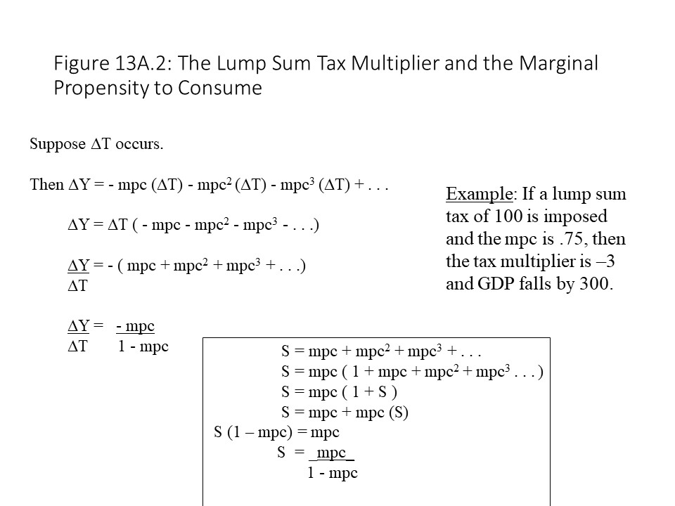
Just as a change in investment spending leads to a multiplier effect as explained in the last section, it is also possible to identify a multiplier effect stemming from the change in lump sum taxes. The reasoning is similar. When taxes are increased, households lose disposable income. They reduce consumer spending, which causes incomes to fall more. The additional reduction in incomes leads to a great drop in consumer spending, and on and on. As before, with each successive round, consumer spending falls by smaller and smaller amounts because not all the lost income would have been consumed anyway at each step.
It is possible to derive a formula that tells us the exact impact that a change in lump sum taxes has on real GDP, other factors held constant. Let’s define the lump sumtax multiplier as the ratio of the change in real GDP to the change in lump sum taxes. By taking into account the way in which the households engage in an infinite series of consumer spending rounds, we can prove that the lump sum tax multiplier is negatively related to the marginal propensity to consume as shown below.
Figure 13A.2 provides the details of the proof for any interested readers. Our main purpose, however, is to understand the intuition behind the formula and to learn how to use it to calculate changes in real GDP. To understand how to use the formula, let’s assume that lump sum taxes rise by 100. If the mpc is 0.75, then we can calculate the lump sum tax multiplier by plugging the mpc into the formula as follows:
Because lump sum taxes rise by 100, we can write the equation as follows:
By solving for the change in real GDP, we can demonstrate that real GDP will fall by $300 billion in this case. Alternatively, the multiplier implies that for every $1 of additional taxes, real GDP will fall by $3. Alternatively, a $1 tax cut would lead to a $3 rise in real GDP. Two points are worth mentioning. First, the lump sum tax multiplier is always negative. The reason is that a rise in taxes causes an opposite change in real GDP. This negative relationship exists because higher taxes reduce consumer spending and lower the equilibrium GDP. Second, the lump sum tax multiplier is smaller in absolute value than the investment multiplier.[9] The reader will recall that the investment multiplier was equal to 4 with the same marginal propensity to consume. The reason for the smaller absolute impact of the lump sum tax multiplier is that when the households receive a lump sum tax cut of, say, $100 billion, they will only spend a fraction of it as determined by the mpc. Successive rounds of additional consumer spending then follow. Conversely, when businesses invest an additional $100 billion, the entire $100 billion is spent in the first round, which then leads to successive rounds of additional consumer spending. Because the initial impact of the additional investment spending is larger than the initial impact of the tax cut, the overall impact of an increase in investment spending is significantly larger than the overall impact of a lump sum tax cut.
Aggregate Demand
Up to this point, we have only considered how the levels of aggregate output and employment are determined. In this section, we want to begin building an explanation of the general level of prices. The aggregate demand/aggregate supply (AD/AS) model was developed for this purpose. The AD/AS model can be understood as an extension of the Keynesian Cross model. We begin by introducing the aggregate demand curve(AD) curve and then explain how it relates to the Keynesian Cross model.
The AD curve, shown in Figure 13.32, asserts that an inverse relationship exists between the general price level (P) and the level of real GDP (Y) that is consistent with equilibrium in the market for goods and services.
The general level of prices may be thought of as a price index such as the consumer price index or the GDP deflator. Even though the AD curve looks much like a market demand curve, it is actually quite different. It turns out that the law of demand does not apply in this context.[10] When we discussed the market demand curve in Chapter 3, it was argued that the market demand curve slopes downward for two main reasons.
First, when the price of an individual commodity falls, consumers substitute away from relatively more expensive commodities whose prices have not changed. This effect, which causes a movement along the demand curve, was referred to as the substitution effect. The downward slope of the AD curve cannot be explained in a similar fashion. When the general price level falls, for example, all commodity prices in the economy are falling and so it does not make sense to talk about substitution away from relatively more expensive domestically produced commodities. It is true that deflation does not necessarily mean that all prices are falling at the same rate. Nevertheless, a drop in a price index does not allow us to detect variation in the reduction of prices across commodities and so this explanation will not suffice as an explanation of the downward sloping AD curve.
Second, when the price of an individual commodity falls, consumers experience a rise in their real incomes. That is, the purchasing power of their nominal incomes increases. Feeling richer, they increased their quantity demanded of the commodity whose price fell as well as the quantities demanded of all other commodities. This effect, which also contributes to the movement along the demand curve, was referred to as the income effect. The downward slope of the AD curve cannot be explained in a similar fashion. When a period of generalized deflation occurs, for example, input prices fall in addition to product prices. The result is that factor incomes decline. With nominal incomes declining along with commodity prices, real incomes are likely to remain the same on average. Therefore, we should not expect an income effect at the aggregate level.
Because the law of demand cannot explain the downward slope of the AD curve, we require a different explanation for its downward slope. To understand its shape, we will first explain the relationship of the AD curve to the Keynesian Cross model. Suppose that the price level falls. We will claim, for reasons not yet explained, that this drop in the price level causes aggregate expenditure to rise as shown in Figure 13.33.
As shown in Figure 13.33, the aggregate expenditures curve shifts upward and raises the level of equilibrium real GDP. The consequence is a negative relationship between the general price level and the level of real GDP. The AD curve thus slopes downward. An explanation must be provided, of course, for the negative relationship between the price level and aggregate expenditure. Neoclassical Keynesian economists provide three main explanations for this negative relationship.[11]
The first explanation for the negative relationship between aggregate expenditures and the general price level is referred to as the wealth effect or the Pigou effect after the classical economist, A.C. Pigou. According to this line of thinking, when the price level falls, even though households do not experience a rise in their real incomes, they do experience a rise in their real wealth. Because other factors are held constant, including nominal wealth (e.g., home prices, stock prices), households experience a rise in the purchasing power of their wealth. As a result, they increase their consumption expenditures, which stimulates aggregate expenditure and raises the equilibrium real GDP. The result is a downward sloping AD curve.
The second explanation for the negative relationship between aggregate expenditures and the general price level is referred to as the international substitutioneffect. According to this line of thinking, when the price level falls, even though no substitution away from relatively more expensive domestically produced commodities occurs, substitution away from relatively more expensive foreign commodities does occur. That is, the drop in the general price level only refers to domestically produced commodities with everything else remaining constant, including prices of foreign commodities. As a result, imports decline and net exports rise. Exports also rise because foreign buyers now substitute towards relatively cheaper commodities in this nation. The aggregate expenditures curve thus shifts upward and the equilibrium real GDP rises. The result is a downward sloping AD curve.
A final explanation for the negative relationship between aggregate expenditures and the general price level is referred to as the interest-rate effect. It is also sometimes referred to as the Keynes effect because Keynes was the first to identify it. According to this effect, when the price level falls, people decide to hold less money because they need less money to engage in transactions. As a result, they lend their excess money holdings, which pushes down the rate of interest. The fall in the rate of interest stimulates investment spending and raises aggregate expenditure. As a result, equilibrium real GDP rises. The result is a downward sloping AD curve.
We are now able to discuss the factors that tend to shift the AD curve. Suppose that for a given price level of P1, the economy is at an equilibrium real GDP of Y1 in the Keynesian Cross model as shown in Figure 13.34.
Now suppose that planned investment spending rises. The aggregate expenditures curve shifts upward, which raises the equilibrium real GDP to Y2. Because the price level has not changed, the equilibrium real GDP will be higher at the same price level in the graph of the AD curve. This change implies a movement off of the AD curve and to the right. Because such movements to the right would occur at any given price level when the level of investment rises, it should be clear that the entire AD curve shifts rightward when investment spending increases. The reader might also note that the AD curve shifts rightward by more than the amount of the increase in investment spending due to the multiplier effect, which is consistent with Figure 13.20. That is, the change in equilibrium output at the current price level more than exceeds the change in investment spending.
Although this example concentrates on a shift of the AD curve due to a change in investment spending, a change in any component of aggregate expenditure will have a similar impact on the position of the AD curve. In general, a rise in consumer spending, investment spending, government spending, or net export spending will shift the AD curve rightward. Similarly, a reduction in consumer spending, investment spending, government spending, or net export spending will shift the AD curve leftward.
To be more specific, consider factors that might influence consumer spending. A rise (fall) in nominal wealth will stimulate (depress) consumer spending and shift the AD curve rightward (leftward). The reader should notice that this effect is not the same as the wealth effect that produced a downward sloping AD curve. The reason is that in this scenario, it is a change in nominal wealth that causes a change in real wealth, rather than a change in the general price level that causes a change in real wealth. Another factor that might alter consumer spending is a change in taxes on household income. If taxes are reduced, then this change will stimulate consumer spending and raise aggregate expenditure. The higher equilibrium real GDP will show up as a shift of the AD curve to the right. A tax increase would have the opposite effects.
Changes in investment spending are likely to have different causes. One major factor influencing investment spending is the rate of interest. If the rate of interest falls, then businesses will borrow more because they are more likely to profit from new investment projects. The rise in investment spending will raise aggregate expenditure and equilibrium real GDP. The result will be a rightward shift of the AD curve. A rise in the interest rate would have the opposite impact and lead to a leftward shift of the AD curve. Other factors that might affect the level of investment include changes in expected profitability. The expected profits from new investment might change to due to changes in the state of the economy, changes in production technology, or changes in business taxes. If business expectations improve, new technologies are developed, or business taxes are cut, then expected profits rise, investment rises, aggregate expenditure rises, and the AD curves shifts rightward. A reduction in expected profits due to the opposite conditions would shift AD to the left.
A change in government spending has a direct effect on the position of the AD curve as well. If government spending rises, then aggregate expenditure rises. The equilibrium real GDP rises, and the AD curve shifts rightward. If government spending falls, then the opposite effects occur, and the AD curve shifts leftward.
A change in net export spending will also influence the position of the AD curve. If trading partners experience economic expansions and incomes are rising, then net exports will rise, raising aggregate expenditures and equilibrium real GDP. As a result, the AD curve will shift rightward. If trading partners experience recessions, then the effects are the opposite and the AD curve shifts leftward. Changes in tariff policy and changes in the foreign exchange value of the domestic currency may also shift the AD curve, although the effects are uncertain due to the possibility of retaliatory tariffs or competitive currency devaluation. Without retaliation, the imposition of tariffs or the devaluation of the currency will discourage imports, raise net exports, raise aggregate spending, and raise equilibrium real GDP. The consequence will be a rightward shift of the AD curve. A reduction in tariff rates or an appreciation of the domestic currency would have the opposite effect if trading partners do not alter their policies, and the AD curve would shift leftward.
Aggregate Supply
Our discussion of aggregate demand has suggested that aggregate spending is the primary determinant of the amount of output produced in the economy. It seems to ignore one other factor that arguably plays a major role in the determination of output: production cost. To capture the role of cost of production in the determination of aggregate output, we turn to the aggregate supply side of the economy. Figure 13.35 shows a graph of the aggregate supply curve(AS) curve.
The graph suggests that a positive relationship exists between the general price level and the level of real GDP that businesses are willing and able to produce at each price level. The aggregate supply (AS) curve looks much like a market supply curve, and the explanation of its shape is similar. That is, as the price level rises, per unit profit rises and so firms expand production, but the increase in production drives up unit costs, which brings the expansion to a halt unless the price level rises further. As production rises, the per unit cost of real output rises due to diminishing returns to labor. The price level must rise to cover the higher per unit cost.
Referring to Figure 13.35, when the economy is operating below the full employment GDP (Yf), increases in real GDP do not put much upward pressure on input prices or unit costs due to the great deal of excess capacity in the economy. As a result, the general price level does not tend to rise much. As the economy approaches the full employment level of GDP, however, efficient resources become more and more difficult to acquire.[12] As a result, less efficient resources must be hired and unit production costs begin to rise. The general price level must, therefore, rise to compensate for the higher unit production costs. That is, businesses raise prices as their production costs per unit increase. A related reason for the rise in per unit production costs as real GDP rises has to do with diminishing returns to labor. With the aggregate stocks of capital and land being relatively fixed during this relatively short time period, the increase in employment raises production but at a decreasing rate. Therefore, it is necessary to hire increasing numbers of workers to raise the production of real GDP by one unit. Hence, unit production costs also rise for this reason and contribute to the upward slope of the AS curve.
The next question that arises deals with the factors that shift the AS curve. Basically, a change in any variable that affects per unit production cost, other than a change in the level of real GDP, will shift the AS curve. A rise in per unit production cost will shift the AS curve to the left because at each level of real GDP, the prices that firms require will need to be higher. A fall in per unit production cost will shift the AS curve to the right because at each level of real GDP, the prices that firms require will be lower. For example, a change in the nominal wage rate will shift the AS curve. It is assumed that when the price level changes, all other variables are held constant, including input prices like wages. If the nominal wage rate rises, then at any given level of real GDP, per unit costs will be higher. The result is a leftward shift of the AS curve as shown in Figure 13.36.
Alternatively, a reduction in the nominal wage would shift the AS curve to the right because per unit cost would be lower at every level of real GDP.
A variety of other factors will also shift the AS curve, but each factor works by influencing the per unit production cost of firms. For example, if the nominal prices of land and capital rise, then the AS curve will shift leftward because unit costs are higher. If other input prices fall, then the AS curve will shift rightward.[13] Factor supplies will also affect the position of the AS curve. If factor supplies (i.e., the supplies of land, labor, and capital) rise, then input prices will fall and the AS curve will shift to the right. If the factor supplies fall, then input prices will rise and the AS curve will shift to the left.[14]
Other factors include the prices of imported inputs.[15] For example, if the price of imported oil rises, then unit production costs will rise and shift AS to the left. If import prices fall, then the AS curve will shift to the right. Changes in the foreign exchange value of the domestic currency will also affect unit cost by making imported inputs more or less expensive. For example, if the domestic currency appreciates, then imported inputs become cheaper for domestic producers. Their unit costs fall, and the AS curve shifts to the right. If the domestic currency depreciates, then imported inputs become more expensive for domestic producers and unit costs rise. The AS curve would then shift to the left.
Changes in labor productivity are also likely to affect unit cost and the position of the AS curve.[16] Labor productivity is measured in terms of output per worker (Q/L) where Q is the number of units of output and L is the number of employed workers. Labor cost per unit may be measured in terms total wages per unit produced (wL/Q) where w is the wage rate. It should be clear that a rise in productivity (Q/L) will cause a drop in labor cost per unit (wL/Q). Hence, a rise in labor productivity will shift the AS curve to the right. If productivity falls, then unit labor cost will rise and shift the AS curve to the left.
The degree of monopoly power in input markets may also influence unit cost.[17] Because monopoly markets produce higher prices than competitive markets, if monopoly power grows in a major input market, then unit costs rise, and the AS curve shifts to the left. If government antitrust action breaks up a monopoly in an input market, on the other hand, then input prices will fall and unit costs will fall as well. The AS curve would then shift to the right.
Finally, changes in business taxes and tax credits may also influence per unit production cost.[18] If business taxes are cut, then unit cost will fall, and the AS curve will shift to the right. If business taxes are increased, then unit labor cost will rise and the AS curve will shift to the left. Alternatively, if the government increases its subsidies or tax credits for business, then in effect unit cost will fall, and the AS curve will shift to the right. If the government cuts its subsidies or tax credits to business then in effect unit cost will rise, and the AS curve will shift to the left.
Macroeconomic Equilibriumand Historical Applications of the Model
Now that the aggregate demand and aggregate supply sides of the model have been developed, we can combine them to explain how macroeconomic equilibrium occurs. Macroeconomic equilibrium occurs when the general price level and the level of real GDP reach levels from which there is no inherent tendency to change. Figure 13.37 depicts an economy that has reached a macroeconomic equilibrium state where P2 and Y2 are the equilibrium general price level and the equilibrium real GDP, respectively.
We want to ask how the economy reaches the equilibrium outcome. It may be tempting to fall back on the explanation that we offered when we discussed the movement to equilibrium in an individual market as in Chapter 3. In this model, however, we need to refer to the factors that cause movements along the AD and AS curves. For example, suppose that the price level is at P3 in Figure 13.37. In this case, aggregate spending is relatively low compared with what businesses wish to produce at this price level. If businesses are producing Y3 and aggregate spending leads to a lower equilibrium GDP in the Keynesian Cross model, then firms will experience a rise in inventories (unplanned investment). They will then cut production. As they cut production, a movement down along the AS curve occurs. The release of relatively inefficient resources causes unit production cost to fall and the price level begins to decline. As the price level falls, three effects on the aggregate demand side occur that stimulate aggregate expenditure. When P falls, households experience a rise in real wealth and consume more. Also when P falls, foreigners begin to buy more of this nation’s exports and domestic buyers buy fewer imports. These factors increase net export spending. Finally, when P falls, the amount of money people wish to hold falls, which leads to more lending, lower interest rates, and higher investment spending. All three factors cause a movement down along the AD curve. Eventually, the economy will arrive at the macroeconomic equilibrium outcome.
Alternatively, suppose that the economy begins with a price level of P1. In this case, businesses do not want to produce much real output given the low price level that just covers their low unit costs. On the other hand, aggregate spending is rather high, leading to a high equilibrium GDP in the Keynesian Cross model. Aggregate output will begin to rise as inventories are depleted as a result of the high aggregate spending. As output begins to rise, the effects of diminishing returns to labor and the employment of less efficient resources causes unit costs to creep upwards. Businesses will raise prices to keep up with rising unit costs. As prices rise, three effects on the aggregate demand side begin to take effect. As P rises, households experience a reduction in their real wealth, which leads to lower consumer spending. As P rises, foreigners substitute away from the nation’s exports and domestic buyers substitute towards imports. Both effects reduce net export spending. Finally, as P rises, people wish to hold more money for transactions purposes and so they lend less. The result is a rise in the rate of interest, which discourages investment spending. All three effects cause a movement up along the AD curve. Eventually, the economy will arrive at the macroeconomic equilibrium outcome.
The AD/AS model can be easily applied to specific periods in U.S. macroeconomic history to obtain a sense of how and why the price level and level of real GDP changed. For example, prior to World War II, the U.S. economy frequently experienced periods of deflation during recessions. The recessions that have occurred since World War II have generally not been characterized by deflation. The AD/AS model can help us to understand why deflation has become less common in the U.S. economy. Figure 13.38 shows a horizontal section of the AS curve, which implies that when AD declines during a recession, the price level does not fall.[19]
During these types of recessions, only real GDP declines. To understand why a horizontal aggregate supply curve might exist, we need to consider how conditions changed in the 1930s and 1940s. In particular, it became more difficult to reduce wages during a recession for a number of reasons, including the passage of a federal minimum wage law in 1938 and the growing power of industrial unions in major industries that negotiated high wage rates. With unit labor costs becoming more rigid, businesses could not reduce them during a recession and so they hesitated to cut prices. Other factors contributing to sticky prices might have been business concerns about menu costs (costs associated with price cuts) and efforts to avoid price wars with oligopolistic competitors.[20] The tendency for prices to be downwardly inflexible means that prices tend to increase, but once they rise, they tend not to fall again.Figure 13.39.
The rise in aggregate demand increased the general price level and the level of real GDP. Because the economy was near the full employment GDP (Y1f), the rise in aggregate demand pushed the unemployment rate below the natural rate of unemployment and had a strong inflationary impact. When inflation is the result of a rise in aggregate demand, economists generally refer to it as a case of demand-pull inflation.[21]
Next let’s consider what occurred in the U.S. during the 1930s. This decade was characterized by a severe reduction in real GDP as well as a falling price level or deflation. The main factor contributing to these changes was a drop in aggregate demand as shown in Figure 13.40.[22]
After the stock market crash of 1929, investment spending and consumer spending fell significantly. The failures of many American banks contributed significantly to the reduction in investment spending as well. As real output fell and unemployment rose, unit costs declined and the price level fell. The price level and level of real output eventually reached P2 and Y2, respectively. If the economy had been subject to downwardly inflexible prices, then the price level would have remained at P1 and the real output would have fallen to Y1. Interestingly, such price stickiness would have made the collapse of output and employment worse during the Great Depression. The falling price level actually took some of the pressure off of real output as aggregate demand fell. The reason that recessions since World War II have been less severe is not the result of sticky prices. Instead, it is because reductions in aggregate demand have been smaller as governments and central banks have become more aggressive about preventing economic collapses.Figure 13.41 shows that a leftward shift of the AS curve was responsible for this inflationary recession.
When inflation occurs at the same time as falling real GDP, the situation is referred to as stagflation. It is the worst of both worlds (i.e., inflation and recession). The reason that the AS curve shifted leftwards in the 1970s had to do with a sudden rise in unit production cost. Unit costs rose because of the two oil price shocks that increased the price of imported oil in the United States. In 1973, the Arab-Israeli War broke out which interrupted the flow of oil to the West. Then in 1979 the revolution in Iran once again led to a disruption of the flow of oil westward. In both cases, tighter global supplies caused the price of oil to skyrocket, raising production costs and leading to stagflation. Because the inflation in this case was the result of an aggregate supply shift, it is often referred to as cost-push inflation to distinguish it from the demand-pull inflation of the 1960s.[23]
Figure 13.42 indicates, both the rise in AD and the rise in AS contributed to a large increase in real GDP. At the same time, only a small increase in the price level occurred because the rise in AS put downward pressure on prices even as the rise in AD tended to push prices up. The economy of this decade was dubbed “The New Economy,” which included the claim that the business cycle had been conquered and that uninterrupted and stable economic growth was to be expected forevermore. The experience of the next decade would serve as a reminder that the business cycle has been far from conquered.[25]
In the year 2000, it became clear that the good times had ended. A stock market bubble had been forming in the IT sector for years. Asset price bubbles form when asset prices rise significantly above levels that are consistent with the real underlying values of the assets. In the case of the IT sector, “irrational exuberance” had led to the bidding up of IT stocks far beyond what would be justified by the profitability of the associated companies. When investors finally discovered to what extent the stocks were overvalued, they dumped them, and the prices collapsed. This disruption in the stock market meant that a great deal of paper wealth was destroyed in a short time. The result was a collapse of investment and consumer spending. Aggregate demand thus fell and gave way to the recession of 2001, like what is depicted in Figure 13.38.
The 2001 recession was mild, however, and the economy soon recovered. The nation’s central bank, the U.S. Federal Reserve, which controls the nation’s money supply, took the lead in responding to the crisis. It increased the money supply which pushed interest rates down to very low levels. As interest rates fell, investment spending rose, but this time investments flowed into the housing sector rather than the IT sector. Over the course of the next few years, a boom in home construction occurred. Low mortgage interest rates encouraged the purchase of new homes, which led to soaring home prices. As before, the bidding upward of these prices above their underlying real values implied the formation of an asset price bubble.
A factor that contributed greatly to the formation of this asset price bubble was the way large financial institutions encouraged the growth of the market for various financial assets, including so-called mortgage-backed securities (MBSs). When commercial banks grant mortgage loans to home buyers, they typically do so for a period of 15 or even 30 years. In the past, a commercial bank would carefully scrutinize the credit worthiness of the home borrower before granting the loan to ensure that the bank would receive mortgage payments each month until the loan was repaid with interest. The growth of the market for MBSs meant that a commercial bank could sell this loan to a large financial institution, like Goldman Sachs, which would then bundle together dozens or even hundreds of such mortgage loans that originated in many different places, creating a single financial asset (i.e., a mortgage-backed security). Goldman Sachs would then sell the MBS to a large institutional investor like a hedge fund. The asset might be sold many times in the organized market for these securities that arose. The owner of the MBS would receive interest payments from many different homeowners due to its ownership of the asset.
The problem that this situation created was that so much money was being made by packaging and selling these specialized assets that less attention was being paid to the credit worthiness of the borrowers. When the loan originator (i.e., the bank that initially grants the loan) is not the same institution that will suffer if the borrower defaults on the loan, it is much less likely that the loan originator will take the proper care in evaluating the credit worthiness of the borrower. Furthermore, credit rating agencies, like Moody’s and Standard and Poor’s, which were supposed to signal to investors how much risk they were assuming by purchasing these securities encountered a conflict of interest. They collected more fees by rating more of these securities. Positive ratings were likely to encourage the growth of the market and keep the market for these securities active. As a result, these agencies tended to be far too optimistic in their valuations and tended to underestimate the degree of risk associated with these securities.
The consequence of all these factors was that home buyers eventually began to default on loans in large numbers. These defaults triggered a collapse in the prices of mortgage-backed securities. Financial institutions that held these assets on their balance sheets watched as the losses mounted. Driven by fear of additional losses, they contracted their lending. The contraction of lending reduced investment spending. Many businesses were unable to obtain the loans necessary simply to pay employees, and business failures began to increase. The result was a huge collapse of aggregate demand as shown in Figure 13.43.
This recession was so extreme that it has been dubbed the Great Recession. It was the worst reduction in real GDP that has occurred since the Great Depression of the 1930s. It should be noted, however, that the Great Depression was far worse with a drop in real GDP and an unemployment rate in excess of 25%. By contrast, during the Great Recession, real GDP fell by just over 4% and the unemployment rate was around 10% at its peak. The reason that the Great Recession was not worse than it was stemmed from the massive government and central bank responses to the crisis. The U.S. Federal Reserve acted as a lender of last resort and offered emergency loans to large financial institutions. The federal government also passed emergency measures, including a $700 billion Troubled Asset Relief Plan (TARP) in late 2008 that bought up hundreds of billions of dollars of so-called toxic assets from banks and other financial institutions while also purchasing equity stakes in the same financial institutions. The federal government also implemented a fiscal stimulus package in early 2009 that included $787 billion of government spending increases and tax cuts. This stimulus package was consistent with the Keynesian prescription for boosting output and employment during recessions. Although these measures had some impact, economic growth remained sluggish for several years and unemployment remained stubbornly high.
The Neoclassical Synthesis Model and the Post-Keynesian Critique
The model that we have investigated up to this point is consistent with the neoclassical interpretation of Keynes’s theory. Keynes’s General Theory is a difficult book and is subject to numerous interpretations. After World War II, Paul Samuelson identified something called the Neoclassical Synthesis model. This model aims to capture what is most valuable in Keynes’s theory while also retaining much of the classical or early neoclassical model that Keynes rejected as incomplete. Because it retains so much of the early neoclassical perspective, many Post-Keynesian economists, who adhere to a very different interpretation of Keynes’s theory, reject the neoclassical synthesis model. We will consider more of the Post-Keynesian perspective in the next chapter. In this section, however, we will briefly consider how neoclassical Keynesian economists aim to create a merger or synthesis of neoclassical and Keynesian ideas.
The proposed merger essentially rests on a distinction between the short run and the long run. As the argument goes, Keynes’s theory best applies to short run changes in aggregate output and employment when nominal wages are sticky. In the long run, however, when nominal wages and other input prices are flexible, it is the classical theory that best applies. To understand this argument, we need to develop a long run aggregate supplycurve (LRAS) curve to distinguish it from the upward sloping short run aggregate supplycurve (SRAS) curve that we have been using throughout this chapter. The LRAS curve is shown in Figure 13.44.
The LRAS curve is perfectly vertical. The reason is that in the long run with perfect price flexibility, all resources will be fully employed. Any unemployment in the markets for land, labor, or capital, will disappear as prices fall and eliminate the unemployment. With each factor of production fully employed, the economy will produce the full employment level of real GDP. Changes in the price level will have no impact on the level of real GDP. The only factors that can shift the LRAS curve are changes in the endowment of society’s resources (i.e., land, labor, and capital) or changes in the available production technology. Otherwise, the LRAS curve will remain where it is.Figure 13.45 where the AD, SRAS, and LRAS curves all intersect to produce an equilibrium price level of P1 and an equilibrium real output of Yf.
Now suppose that the central bank increases the money supply, which pushes the interest rate down and stimulates investment spending. The rise in investment spending increases aggregate demand, shifting the AD curve to the right. According to Keynesian theory, output rises above the full employment level to Y2 and the unemployment rate falls below the natural rate of unemployment. At the same time, the price level rises to P2 due to the rise in per unit cost. The Keynesian short-run explanation would stop at this point, but according to the neoclassical synthesis model, in the long run factor prices will begin to rise. As nominal wages and other factor prices rise pushing up unit cost, the SRAS curve shifts to the left. The new long run equilibrium then occurs at the intersection of AD, the new SRAS curve, and the LRAS curve. Output returns to the long run level, and the price level is permanently higher at P3. Even though Keynes’s theory provides an explanation for the short run fluctuations, the classical theory provides the long run explanation.
Of course, Post-Keynesian economists are highly critical of the neoclassical synthesis model. The model assumes that if we wait long enough, then wages will adjust to bring about full-employment. It was precisely this kind of thinking that Keynes rejected in his General Theory. Keynes’s famous remark in response to such thinking was that, “In the long run, we are all dead.” Furthermore, this particular example suggests that money is not neutral in the short run, but it is neutral in the long run. Those who defend the neutrality of money argue that changes in the money supply cannot cause changes in real variables, like output and employment. Post-Keynesian economists have long argued that Keynes’s theory implies the non-neutrality of money in both the short run and the long run. More will be said about the Post-Keynesian perspective in later chapters.
A news article published in EIU ViewsWire describes how changes in the foreign exchange value of the Icelandic Krona have affected Iceland’s economy since the global financial crisis of 2008. The article explains how the Krona approached new lows after the financial crisis, which supported “a boom in the tourism industry that drove the post-crisis recovery in the Icelandic economy.” In terms of the AD/AS model, the depreciating Krona helped stimulate aggregate demand. When a nation’s currency depreciates, a nation’s exports become cheaper and its imports become more expensive. The consequence is a rise in net exports and an increase in aggregate demand. Real output and employment should then rise, as occurred in the case of Iceland. The article explains that eventually the improved performance of the economy led to a higher demand for the Krona, which caused it to steadily appreciate in 2014-2015 and then significantly more in 2016. The article explains that the Icelandic low-cost airline, Wow Air, faced increasing competitive pressure as a result of the appreciating Krona, and that the weak financial performance of Iceland’s airlines was beginning to have a negative effect on the tourism industry. As investors became cautious about Iceland’s future growth prospects, the exchange value of the Krona began to slide, leading to a sharp depreciation of the Krona, which fell by roughly 10% against the Euro between August and October 2018, as the article explains. In response to the depreciation of the Krona, the Central Bank of Iceland has been increasing interest rates. Higher interest rates should encourage investors to purchase interest-bearing assets in Iceland, which will help the Krona recover. As a result, the author of the article expects upward pressure on the Krona throughout 2019. Although a currency depreciation tends to simulate aggregate demand, the article explains that the central bank has been raising interest rates because it is concerned about the higher prices of oil imports and increases in labor costs due to an upcoming round of collective wage negotiations. Higher oil prices and high labor costs both reduce aggregate supply, which can be inflationary and can cause a reduction in real output, as the AD/AS model implies. Therefore, a currency appreciation can be beneficial to producers because it lowers the prices of imported inputs and may increase aggregate supply. The AD/AS model shows us the various ways that a change in the foreign exchange value of a nation’s currency might affect its economy.
Summary of Key Points
Say’s Law of Markets states that new production will always generate enough income for its purchase and so general gluts of overproduction are not possible in market capitalist economies.
According to J.M. Keynes, Say’s Law of Markets does not hold in market capitalist economies because not all savings will be invested.
The consumption function and the saving function show that consumer spending and saving are positively related to the disposable income of households.
The Keynesian Cross model explains how the economy arrives at an equilibrium level of real GDP as businesses change production in response to a buildup or depletion of inventories.
In the Keynesian Cross model, the equilibrium condition states that aggregate planned expenditure is equal to real GDP.
The paradox of thrift asserts that even if all households increase their saving, aggregate saving will ultimately not change.
The Keynesian multiplier effect refers to the tendency for real GDP to rise by a multiple of a rise in investment spending.
In the Keynesian Cross model, trade surpluses raise equilibrium GDP, trade deficits reduce equilibrium GDP, and balanced trade leaves equilibrium GDP unchanged.
In the Keynesian Cross model, government spending increases or tax cuts raise equilibrium real GDP, whereas government spending reductions or tax increases reduce equilibrium real GDP.
The lump sum tax multiplier is negative and has a smaller absolute impact on real GDP than the investment multiplier.
The AD curves slopes downward due to the wealth effect, the international substitution effect, and the interest-rate effect.
The AD curve shifts due to changes in consumer spending, investment spending, government spending, and net exports.
The AS curve slopes upward due to rising unit costs as less efficient resources are employed and diminishing returns to labor occurs.
The AS curve shifts due to changes in all other factors that affect unit costs, such as changes in input prices, import prices, the exchange rate, business taxes and credits, monopoly power, labor productivity, and input supplies.
Macroeconomic equilibrium occurs at the intersection of the AD and AS curves and determines the equilibrium real GDP and price level.
The neoclassical synthesis model represents a merger of neoclassical economics and Keynesian economics.
List of Key Terms
Say’s Law of Markets
Aggregate production function
Consumption function
Autonomous consumption
Marginal propensity to consume (mpc)
Saving function
Autonomous saving
Marginal propensity to save (mps)
Reference line
Keynesian Cross model
Aggregate expenditures model
Induced spending
Planned investment
Actual investment
Paradox of thrift
Induced saving
Fallacy of composition
Multiplier effect
Animal spirits
Trade surplus
Trade deficit
Balanced trade
Tariff
Competitive devaluation
Mixed economy
After-tax consumption function
Pre-tax consumption function
Lump sum tax multiplier
Aggregate demand (AD) curve
Substitution effect
Income effect
Wealth effect
International substitution effect
Interest-rate effect
Aggregate supply (AS) curve
Macroeconomic equilibrium
Sticky prices
Menu costs
Demand-pull inflation
Stagflation
Cost-push inflation
Asset price bubbles
Mortgage-backed securities (MBSs)
Great Recession
Neoclassical Synthesis model
Long run aggregate supply (LRAS) curve
Short run aggregate supply (SRAS) curve
Neutrality of money
Problems for Review
1.Suppose the consumption function is C = 250+0.8DI. What is the saving function?
2. Suppose that investment spending falls by $300 billion. If the mpc is 0.6, then what is the change in real GDP, according to the Keynesian multiplier effect?
3. Suppose you are given the following information about the economy:
Investment spending is 400
Government spending is 600
A trade deficit of 250 exists
Autonomous consumption is 300
The mpc is 0.70
A lump sum tax of 275 is imposed
Given this information, write the aggregate expenditures function. Then calculate the equilibrium level of real GDP and place your answer on a graph like the one below. 4. Suppose that a lump sum tax cut of $125 is imposed on households. If the mpc is 0.82, then what will be the overall change in real GDP that results?
5. Suppose that the economy begins in macroeconomic equilibrium as depicted in the AD/AS model. Suppose that a stock market collapse occurs that reduces household wealth at the same time that monopoly power increases in key input markets. What will happen to the equilibrium levels of prices and real GDP? Represent your answer graphically.
6. Suppose that the economy begins in macroeconomic equilibrium as depicted in the AD/AS model. Suppose that the domestic currency depreciates. What will happen to the equilibrium levels of prices and real GDP? Consider the impact on both AS and AD in your answer. Represent your answer graphically.
7. Suppose that the economy begins in macroeconomic equilibrium as depicted in the AD/AS model. Suppose that labor productivity rises at the same time that taxes on households are reduced. What will happen to the equilibrium levels of prices and real GDP? Represent your answer graphically.
See Snowdon, et al. (1994), p. 44-51, for a more advanced treatment of the classical model of output and employment. ↵
See Hunt (2002), pp. 405-408, for a discussion of how Keynes’s theory relates to the neoclassical flow model. ↵
Hunt (2002), pp. 413-415, graphically represents the two major causes summarized here. ↵
See Wolff and Resnick (2012), p. 106-107, for a discussion of how Keynes introduced this new entry point. ↵
See Wolff and Resnick (2012), p. 40-41, for a discussion of the logic of Keynesian theory. ↵
See Chiang and Stone (2014), p. 507-509, for the conditions under which saving ends up falling overall. ↵
See U.S. Bureau of the Census (1975), Series U 187-200. Value of Exports and Imports: 1790 to 1970, p. 884-885. The calculation of the trade balance includes total merchandise, gold, and silver. ↵
Hubbard and O’Brien (2019), p. 792-793, emphasize differential growth rates across countries, differential price levels across countries, and exchange rates as the major factors influencing the level of net exports. McConnell and Brue (2008) also emphasize tariffs. ↵
See Samuelson and Nordhaus (2001), p. 504-505, who make this point in the context of an example where a tax increase is required to balance the government budget after a government spending increase. ↵
Chiang and Stone (2014), p. 524, and McConnell and Brue (2008), p. 188, argue that neither the income effect nor the substitution effect can explain the downward slope of the AD curve. See also Case, Fair, and Oster, p. 550. ↵
These effects are identified in nearly all neoclassical textbooks when the downward sloping AD curve is explained. ↵
OpenStax (2014) refers to firms “running into limits” as the economy approaches its potential GDP. ↵
Many textbooks mention changes in commodity prices and changes in nominal wages. See Krugman et al. (2014), p. 422. ↵
Hubbard and O’Brien (2019), p. 834, emphasize changes in the labor force and capital stock. Other books such as OpenStax (2014) describe these changes as supply shocks. ↵
Prices of imported inputs are also frequently mentioned in textbooks. See OpenStax (2014), p. 562, and Samuelson and Nordhaus, p. 662. ↵
See OpenStax (2014), p. 560-561, and McConnell and Brue (2008), p. 195, for a discussion of how productivity changes can influence the AS curve. ↵
McConnell and Brue (2008), p. 198, analyze the post-WWII recessions in this way. McConnell and Brue (2008), p. 198, and OpenStax (2014), p. 588, provide similar graphs representing this scenario. ↵
McConnell and Brue (2008), p. 199, include such arguments. Similar arguments may also be found in OpenStax (2014), p. 585. OpenStax (2014), p. 585, also mentions a coordination argument that Keynes made. That is, although workers might accept a wage cut if all workers simultaneously received one, coordinating an economy-wide wage cut is not possible in a decentralized market economy. ↵
The case of demand-pull inflation is a common one in neoclassical textbooks. See Chiang and Stone (2014), p. 536-537, Samuelson and Nordhaus (2001), p. 425-426, and Bade and Parkin (2013), p. 760. ↵
See Coppock and Mateer (2014), p. 436, for a similar representation of this case. ↵
The case of cost-push inflation is also a common one in neoclassical textbooks. See Chiang and Stone (2014), p. 537-539, Samuelson and Nordhaus (2001), p. 426-427, and Bade and Parkin (2013), p. 761. ↵
McConnell and Brue (2008), p. 200-202, analyze this case. It is also included as an exercise in Krugman et al. (2014), p. 445. Hubbard and O’Brien (2019) analyze the case too but without emphasis on the low inflation rates. ↵
McConnell and Brue (2008), p. 202, make this connection to the “New Economy.” Interestingly, history has repeated itself. In the 1920s, many respected observers claimed that a “new economics” had abolished the business cycle thanks to the establishment of the Federal Reserve in 1913. See Chancellor (1999), p. 192. ↵
“Iceland economy: Sharp depreciation in the krona prompts policy action.” EIU ViewsWire. The Economist Intelligence Unit N.A., Incorporated. New York. 10 Nov. 2018. ↵


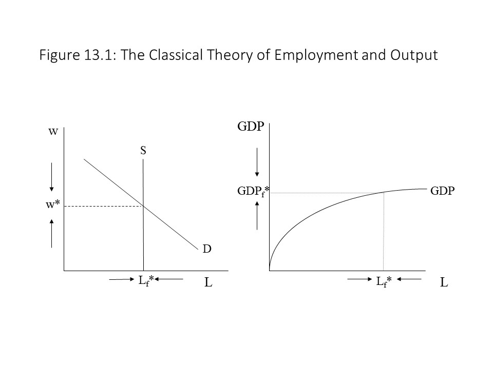 If the market wage (w) is above the equilibrium wage (w*), then a surplus of labor or unemployment exists. Competition will force the market wage down until the market wage coincides with the equilibrium wage. The surplus will be eliminated and the quantity of labor demanded will equal the available labor force (Lf*). With the economy operating at full employment, the economy will be able to produce at the full employment level of GDP (GDPf*). The full employment GDP is shown in Figure 13.1 using the aggregate production function. The aggregate production function exhibits diminishing returns to labor, which assumes that all other factors of production (e.g., land and capital) are held constant. Of course, all available land and capital will be fully employed as well, assuming that the markets for these resources have cleared as well. Given the available production technology and the fully employed resources, the economy will produce the potential GDP.
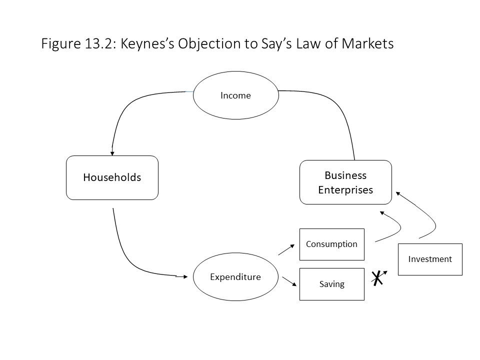 As Figure 13.2 shows, business enterprises make payments to households in exchange for the resources households sell to businesses. Households receive factor income for the land, labor, and rent that businesses purchase. The businesses use these factors of production to produce finished commodities. The households then spend this factor income on the finished commodities, but it is here that we deviate from our earlier discussion of the neoclassical circular flow model from Chapter 3. Obviously, households will choose to save some of their income and not spend it. The classical economists and early neoclassical economists understood this point well. They argued that the saving that occurred would flow into the loanable funds market where it would be transferred to individuals and firms who would invest it. These investments in new capital goods would add to the demand for consumer goods and ensure that all of the finished commodities were sold. Of course, these borrowers would pay interest to the lenders for the use of the borrowed funds, but the circular flow would be maintained and Say’s Law would hold.
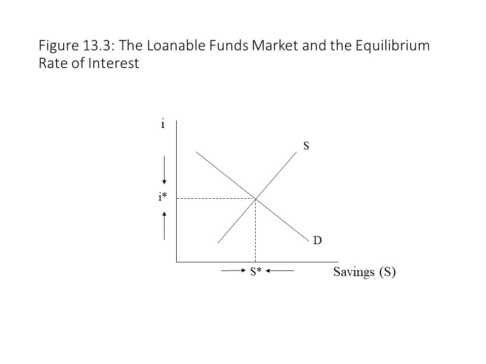 If a surplus of savings exists, then in the classical theory, the market rate of interest (i) will fall to the equilibrium level of i* and clear the loanable funds market. Aggregate saving will equal aggregate investment. If, however, other forces are acting on the rate of interest that prevent it from falling, then the surplus of savings will persist and not all savings will be invested. As a result, not all finished commodities will be sold due to insufficient investment demand. Alternatively, it might be that the market clearing level of the rate of interest (i*) does not occur at a market rate of interest that is greater than or equal to zero due to a very large supply of savings and a relatively low level of investment demand. In that case, the market rate of interest will not be able to fall enough to clear the market for loanable funds and the surplus of savings will persist. In this case as well, an excess supply of finished commodities or a glut will occur. The result will be falling production as firms scale back production, falling employment as they lay off workers, and falling prices due to the excess supplies of commodities. All these results were observed during the Great Depression, which is exactly what Keynes developed his theory of effective demand to explain with the hope of ending depressions by means of enlightened government economic policy.
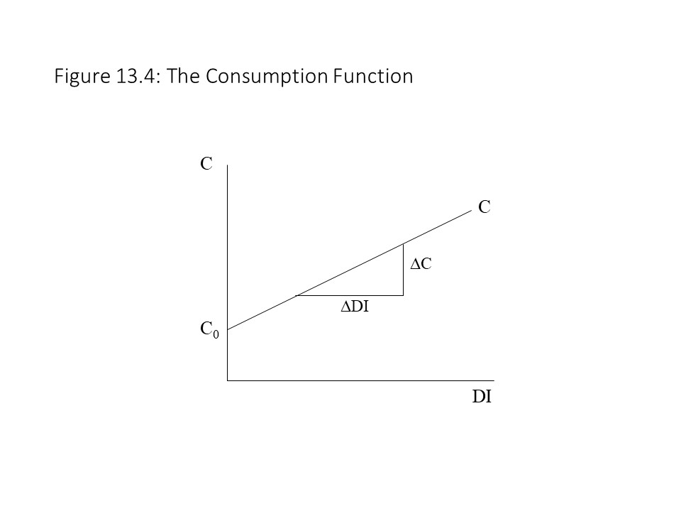 Because the mpc is assumed to be fixed at every level of DI, the slope is constant and the consumption curve graphs as a straight line. To consider a simple example, suppose that the consumption function is C = 200+0.75DI. In this case, even if DI is equal to zero, the households will spend $200 billion. Also, for every $1 of additional DI that the households receive, they will consume an additional $0.75.
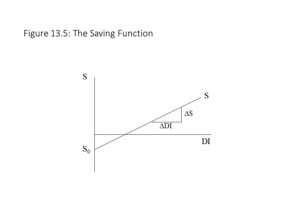 Because the mps is assumed to be fixed at every level of DI, the slope is constant and the saving curve graphs as a straight line. To consider a simple example, suppose that the saving function is S = -200+0.25DI. In this case, even if DI is equal to zero, the households will save -$200 billion. Also, for every $1 of additional DI that the households receive, they will save an additional $0.25.
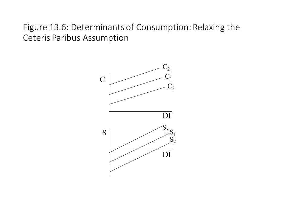 One should also consider the relationship between the mpc and the mps. Suppose we add the two measures together as follows:
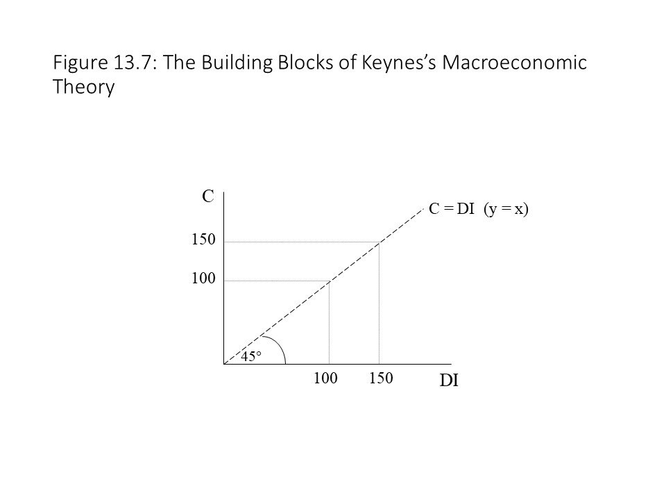 As Figure 13.7 indicates, at each level of DI, the level of C that corresponds to it is found on the reference line. That is, the horizontal distance to that level of DI will be exactly the same as the vertical distance from that level of DI up to the 45 degree line. Another way to think about this reference line is that it has a slope equal to 1 and a vertical intercept equal to zero, much like the equation y = x in the case that y is placed on the vertical axis and x is placed on the horizontal axis.
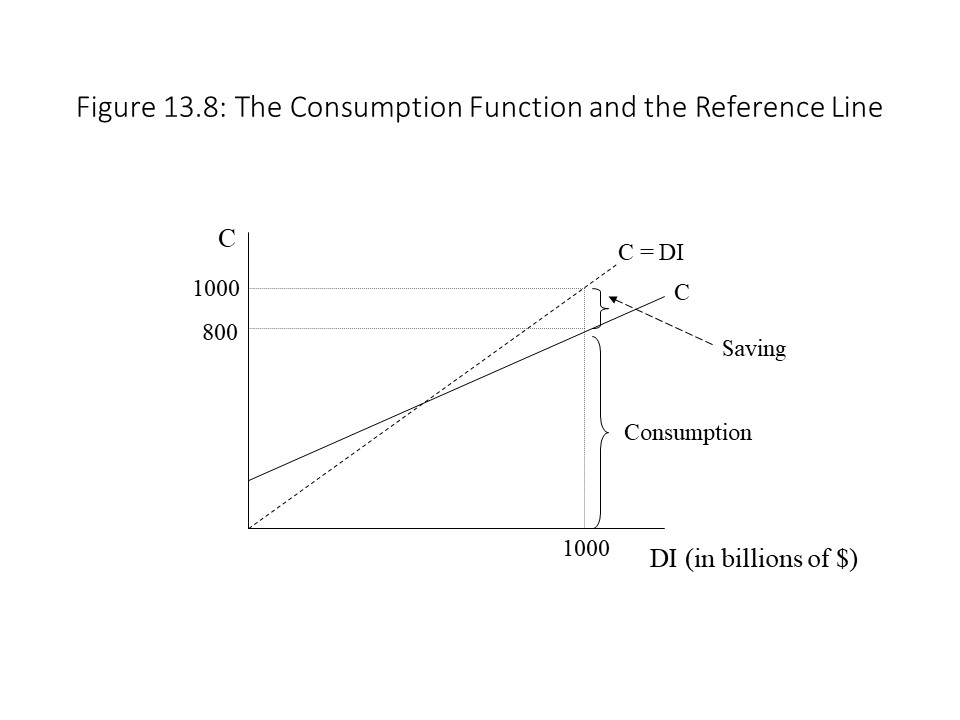 As Figure 13.8 shows, at a level of DI of $1000 billion, the reference line allows us to represent that amount vertically. It is then much easier to see which part of the DI is spent on consumption and which part remains for saving. In this case, $800 billion is consumed and $200 billion is saved. In general, at every level of DI at which the C line is below the reference line, positive saving exists. The reader will notice that the lines intersect at a single point. At this point, planned consumer spending equals DI, which is true for all points on the reference line. When planned consumer spending equals DI, we refer to this income level as the break-even income level. In other words, households have just enough DI to finance their consumption expenditures, no more and no less. Finally, if DI is at a low enough level that the C line is above the reference line, then planned household consumption expenditures exceed DI and the households must be borrowing or relying on past savings to finance the excess consumption.
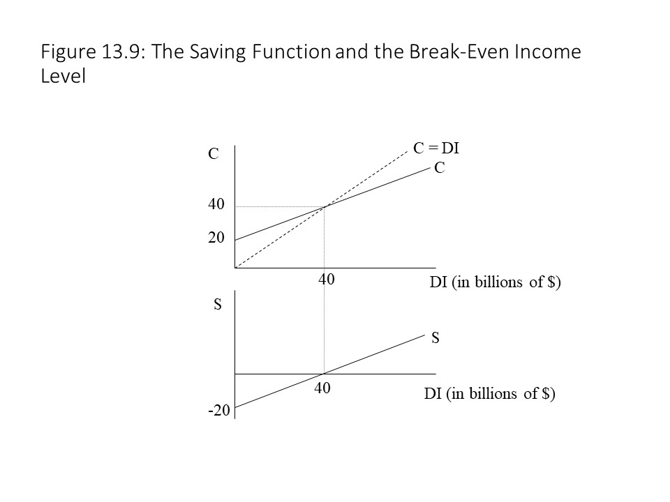 At the break-even income level of $40 billion in the top graph, C = DI and thus S = 0. Therefore, the bottom graph shows the saving function crossing the DI axis at $40 billion, indicating a level of saving equal to zero at that level of DI. As we move to the right of the break-even income level in the top graph, we see that saving becomes positive and continues to grow as the gap between the two lines becomes larger. Therefore, in the bottom graph, the level of saving becomes positive and continues to grow when DI rises above $40 billion.
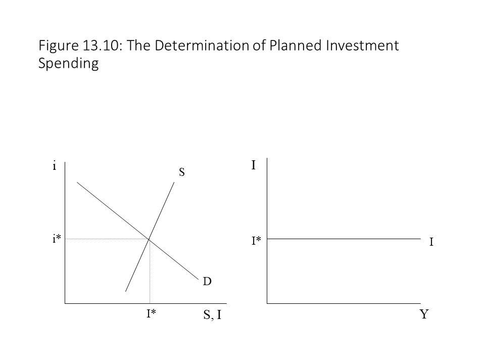 As the reader can see in the graph on the right, investment spending (I) is equal to IO and is thus constant at all levels of real GDP (Y).
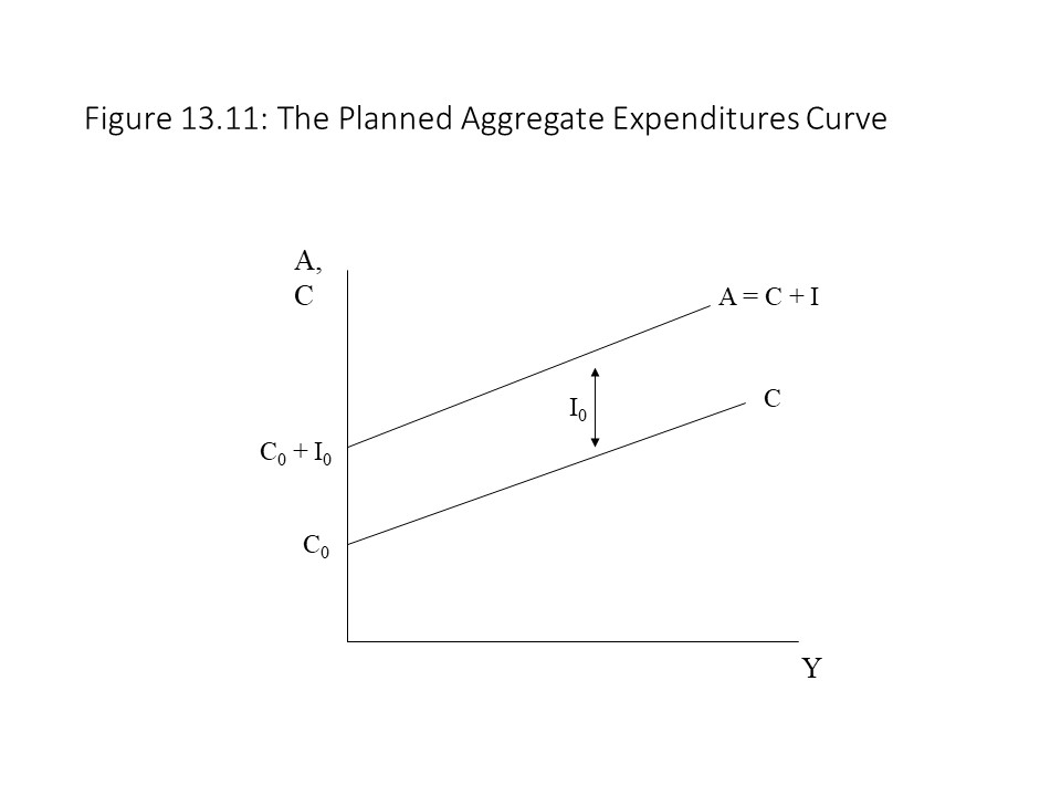 As the reader can see, the planned aggregate expenditures curve has a vertical intercept equal to the level of autonomous spending. The vertical distance between A and C is constant and equal to IO at every level of DI. The slope of the aggregate expenditures curve is also equal to the mpc because the A and C curves are parallel to one another.
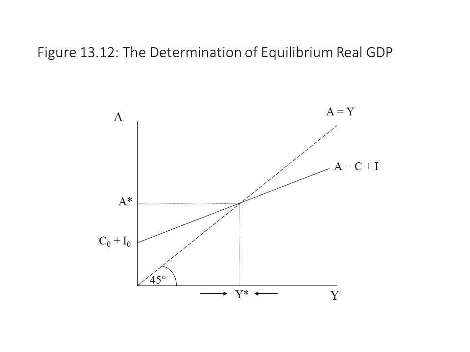 At this point, planned aggregate spending equals real aggregate output and so all plans are perfectly satisfied by the level of production. The reason this level of real GDP is the equilibrium level can be understood by considering what will occur if the economy is not producing at this point. Suppose that the level of real output is above Y* in the graph. In that case, planned aggregate spending is below the level of real output as shown on the 45-degree line. That is, A < Y. As a result, firms will be producing more than households and firms wish to purchase. As a result, business inventories will build up as a result of the excess supply of commodities. The consequence will be a drop in the level of production as firms cut production. Real GDP will then fall towards the equilibrium level. Conversely, if the level of real GDP is below Y* in the graph, then planned aggregate spending is above the level of real output as show on the 45-degree line. That is, A > Y. As a result, firms will be producing less than households and firms wish to purchase. As a result, business inventories will be depleted as a result of the excess demand for commodities. The consequence will be a rise in the level of production as firms raise production. Real GDP will then rise towards the equilibrium level.
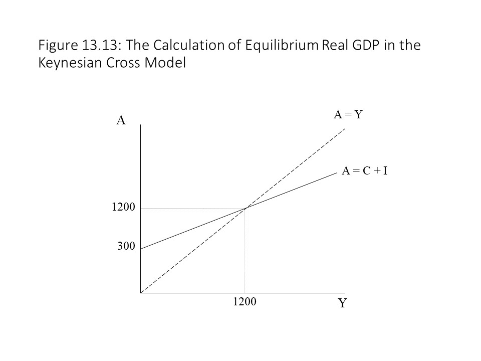 The graph shows that the equilibrium level of real GDP occurs at the intersection of the reference line and the planned aggregate expenditures curve. Solving the two equations simultaneously yields the solution.
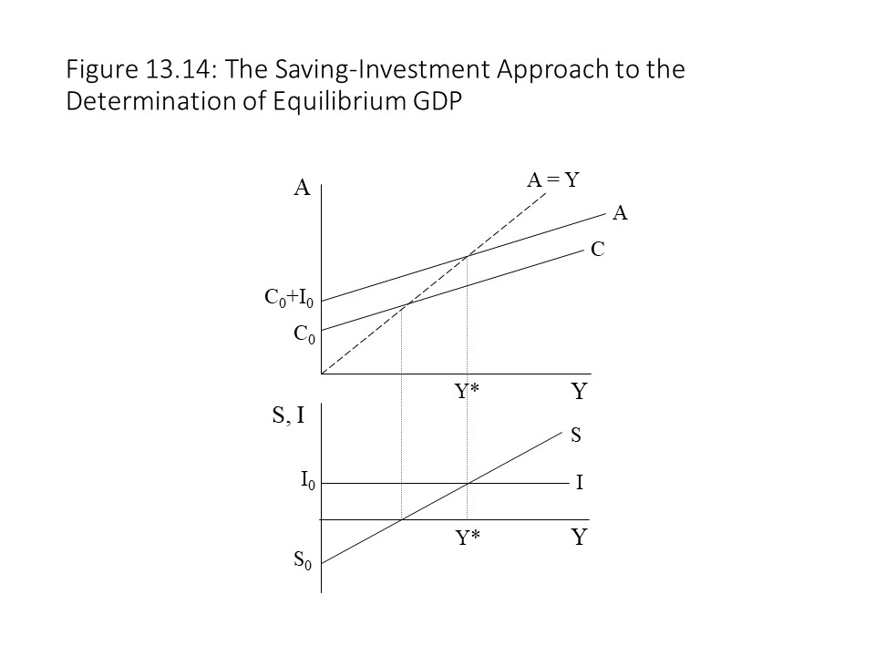 Because planned investment is constant at all levels of GDP, it is represented as a horizontal line in the graph. The saving curve, on the other hand, slopes upward for reasons already discussed. The equilibrium level of real GDP occurs at the intersection of the two lines.
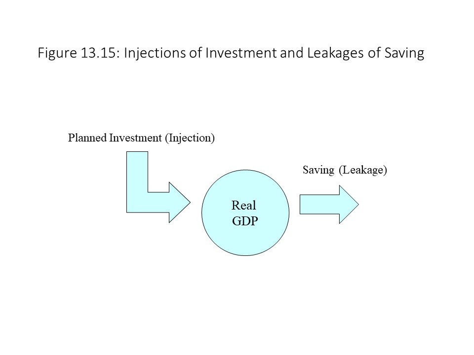 In Figure 13.14, if the level of real GDP is below the equilibrium level of Y*, then planned investment exceeds saving. With the injection larger than the leakage, the result is a rise in real GDP and a movement towards the equilibrium level. On the other hand, if the level of real GDP is above the equilibrium level of Y*, then saving exceeds planned investment. With the leakage larger than the injection, the result is a fall in real GDP and a movement towards the equilibrium level.
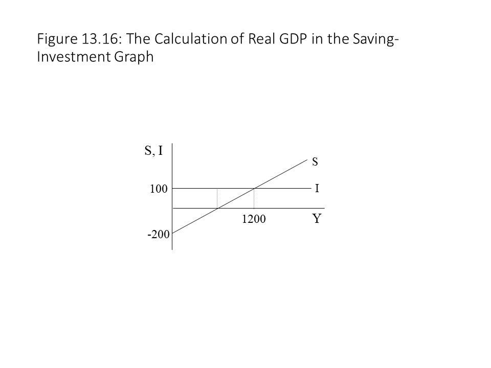 The reader might be a bit confused by the claim that saving equals investment only in equilibrium. After all, it was argued in Chapter 12 that GDP is always equal to the sum of consumer spending, investment spending, government spending, and net export spending. In a closed, private economy without government spending or net exports, GDP should always equal consumer spending plus investment spending. Therefore, if GDP is the sum of consumer spending and saving, then saving should always equal investment spending. The reason for the apparent contradiction is that the equilibrium condition only refers to planned investment whereas the measurement of GDP includes actual investment. In other words, saving will always equal actual investment, which includes both planned investment spending and inventory (unplanned) investment spending. At the same time, saving may not equal planned investment spending. Figure 13.17 clarifies this point.
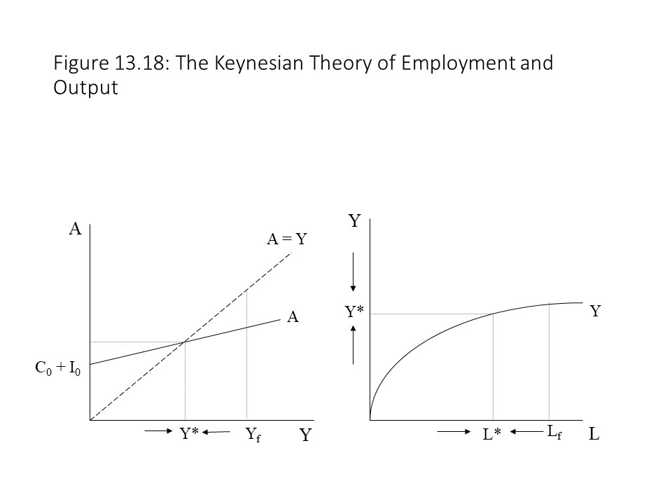 Furthermore, as businesses adjust production in the movement to equilibrium, they also adjust their workforces. Employment, therefore, moves towards an equilibrium level of L* that corresponds to the equilibrium level of real GDP as shown on the production function. Employment also ends up below the full employment level of Lf. Hence, Keynes’s theory is one of unemployment equilibrium, and it reveals the case of full employment GDP to be a special case. That is, aggregate planned spending would need to be just high enough to produce the full employment GDP as the equilibrium GDP. Keynes could, therefore, argue that his theory was a more general theory than the classical theory of employment and output.
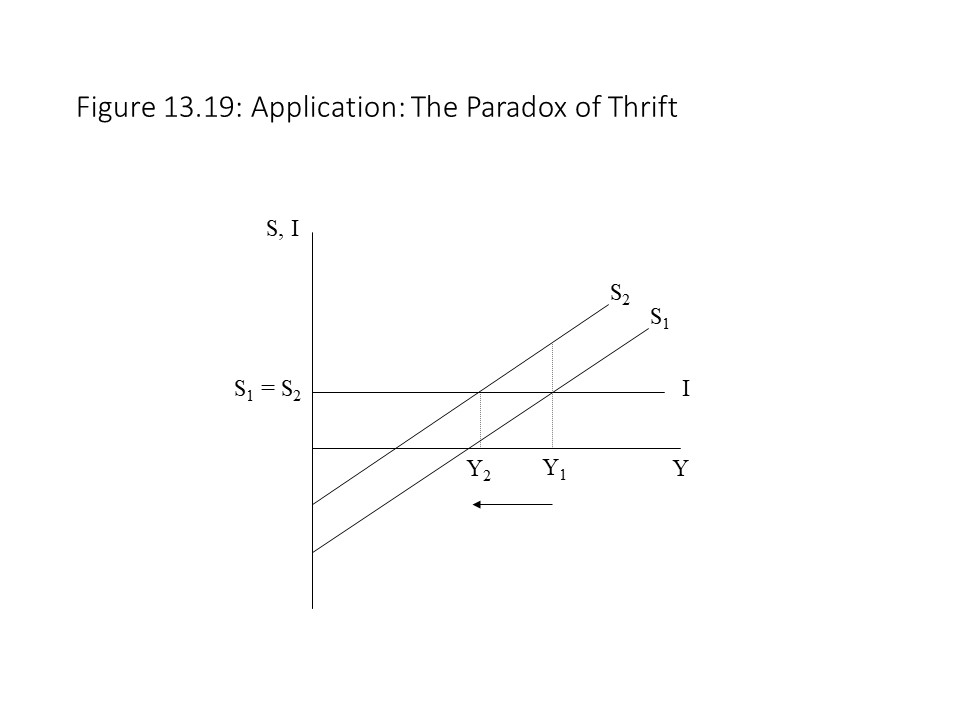 Initially, saving rises at Y1, but this increase in saving causes a discrepancy between saving and planned investment spending. Specifically, saving rises above planned investment spending. With the leakage of saving being higher than the injection of planned investment, real GDP begins to fall. The drop in real GDP causes a movement along the new saving curve. In other words, induced saving declines. The reduction in saving continues until it once again equals planned investment and the economy returns to equilibrium at Y2. The problem for the economy is that the high level of saving has led to a recession (i.e., falling real GDP) rather than to economic growth, as suggested by the production possibilities model. Furthermore, and rather paradoxically, even though all households decided to save more, aggregate saving returns to the same level that previously existed.[6] The reason is that the recession has led to falling incomes, which reduces saving.
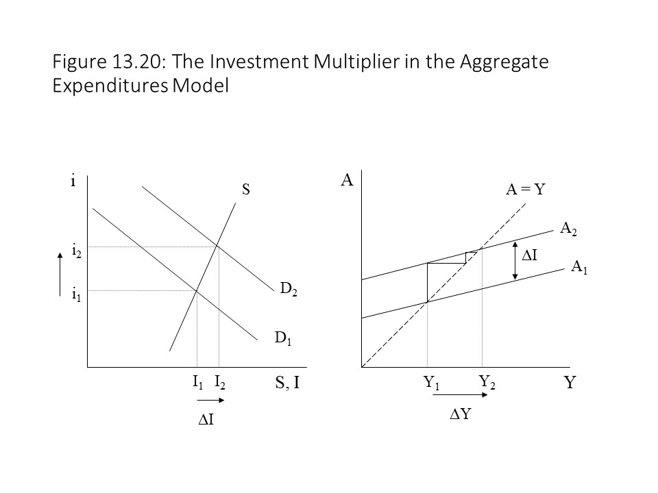 The rise in planned investment raises the aggregate expenditures curve as shown in Figure 13.20. The result is a higher level of equilibrium real GDP and the economy experiences an economic boom. Interestingly, the graph on the right in Figure 13.20 suggests that the level of real GDP rises by more than the rise in planned investment. Because the slope of the reference line is equal to 1 and the difference between the old and new A curves is equal to the change in planned investment, the first move up along the reference line would indicate a rise in real GDP equal to the rise in planned investment spending. As the reader can see in the graph, however, real GDP rises by more than this amount. Hence, a multiplier effect is implicit in the Keynesian Cross model.
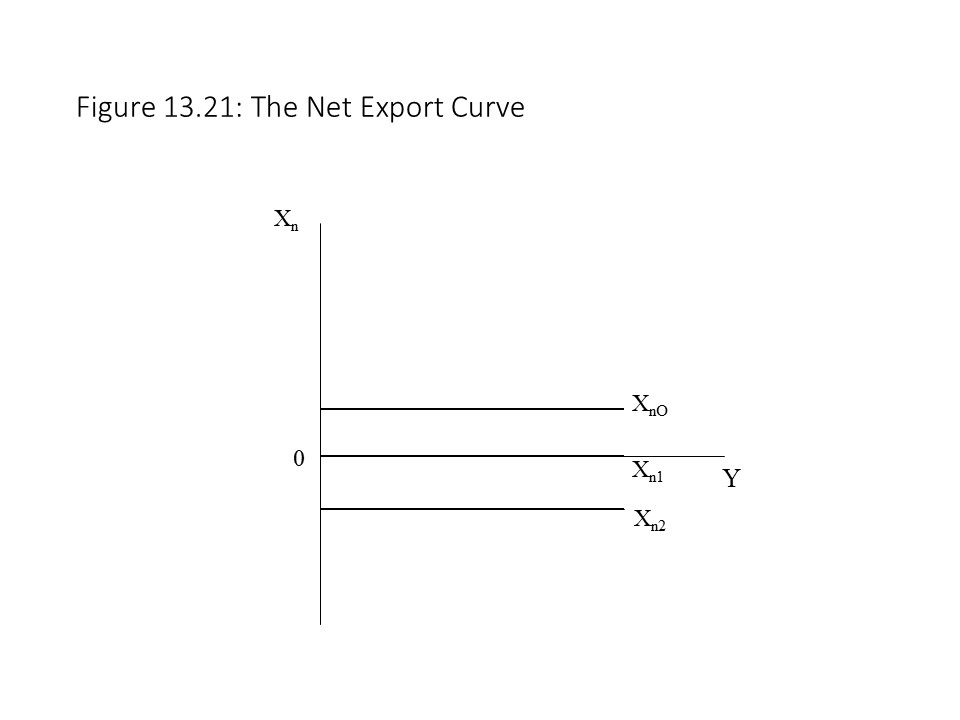 As Figure 13.21 shows, net exports may be positive (XnO), equal to zero (Xn1), or negative (Xn2). The reader should recall that net exports equal exports (X) minus imports (M). As explained in Chapter 12, if net exports are positive, then a trade surplus exists (X > M). If net exports are negative, then a trade deficit exists (X < M). If net exports are equal to zero, then balanced trade exists (X = M).
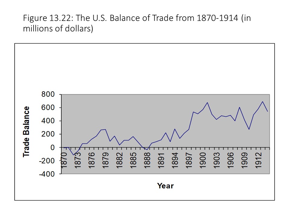 In the Keynesian Cross model, we can now add net exports to the consumption function and level of planned investment spending to obtain the aggregate expenditures function as follows:
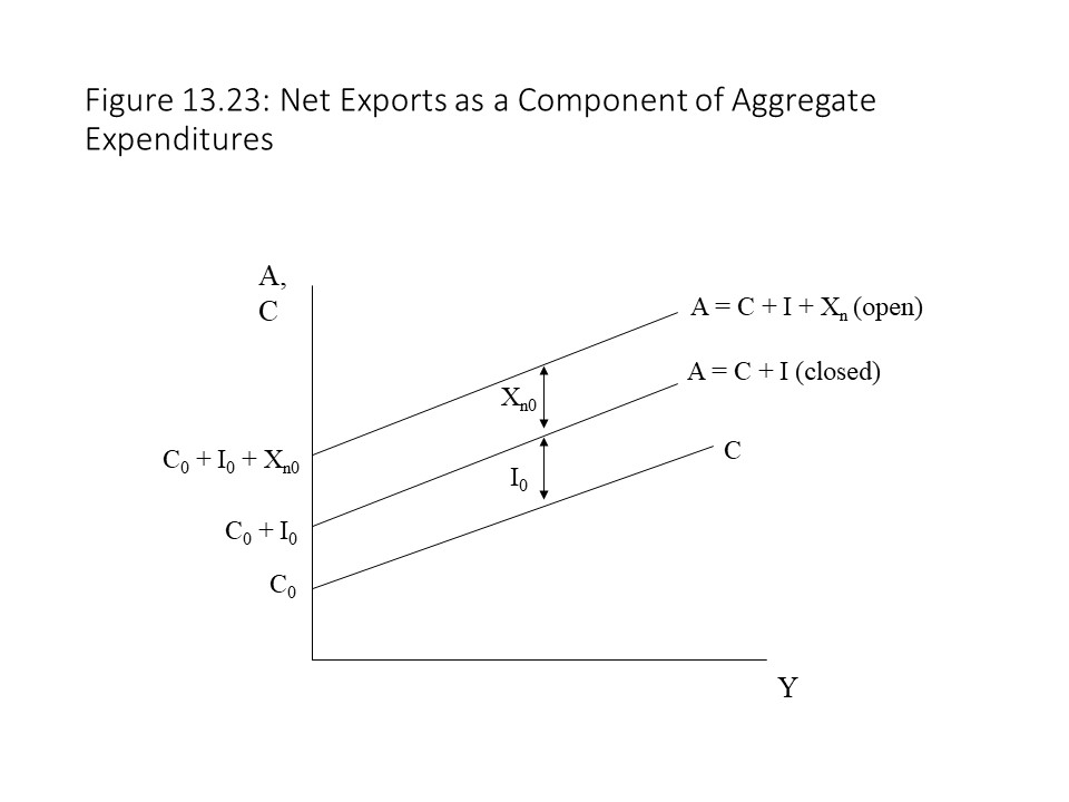 As the figure shows, the opening of the economy shifts the aggregate expenditures curve upward due to the trade surplus that results.
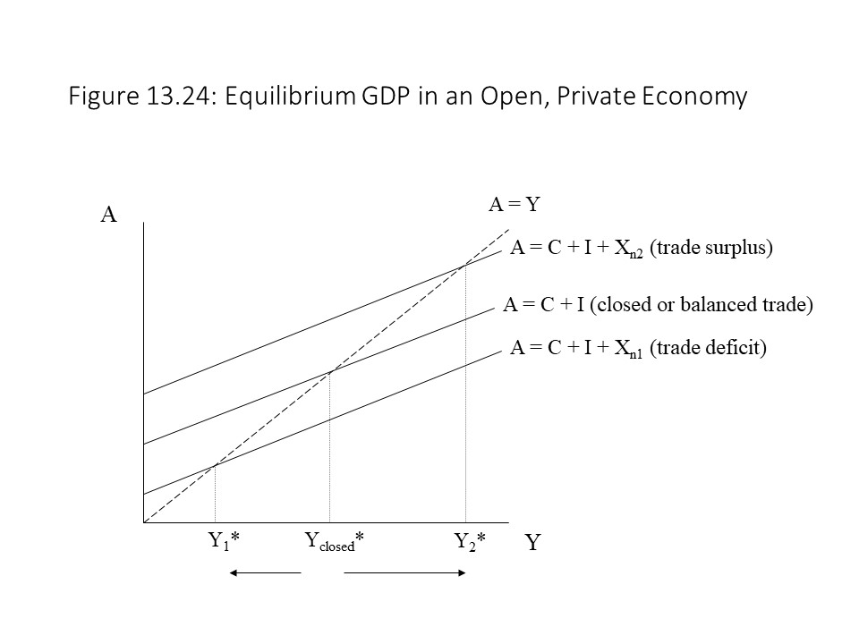 As Figure 13.24 shows, a trade surplus raises the aggregate expenditures curve and increases the equilibrium real GDP. A trade deficit, on the other hand, lowers the aggregate expenditures curve and reduces the equilibrium real GDP. Balanced trade leaves the aggregate expenditures curve unchanged and leaves the equilibrium real GDP unchanged. The case of balanced trade demonstrates that the spending by foreigners on the economy’s exports is exactly canceled by the spending of domestic buyers on imports from other countries in terms of the impact on real GDP. This analysis also allows us to draw a conclusion about the desirability of a trade surplus and the disadvantage of a trade deficit. Trade deficits appear to be harmful because they lower the nation’s equilibrium real GDP and employment level. Trade surpluses, on the other hand, appear to be beneficial because they raise the nation’s aggregate output and employment.
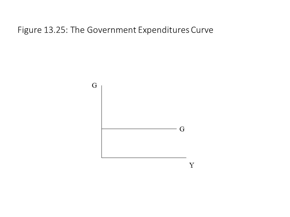 Government spending is assumed to be determined by legislators and a whole host of political factors that neoclassical Keynesian economists do not attempt to explain. Nevertheless, we can now add government spending to the consumption function, the level of planned investment spending, and the level of net exports to obtain the aggregate expenditures function as follows:
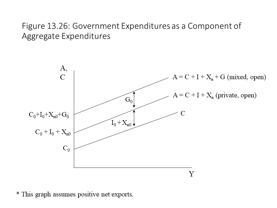
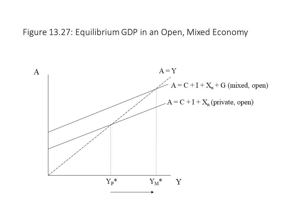 It should be rather obvious now why Keynes advocated increased government spending during the Great Depression. By increasing government spending, it is possible to increase aggregate output and employment. With a purely private economy stuck at an unemployment equilibrium, government spending can move the economy closer to full employment. Alternatively, reducing government spending during a recession would only worsen the situation by reducing aggregate output and employment in an already weak economy.
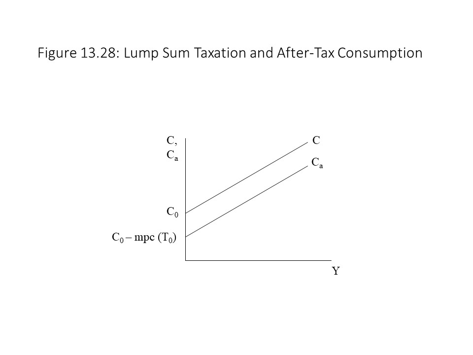 The reason that the lump sum tax lowers consumption at every level of real GDP by this amount is that the households lose the tax amount as part of their income. Because households consume part of their income and save part of their income, when they lose the tax amount, they reduce their consumption by the amount that would have been consumed had they been able to keep this income. That is, they reduce their consumption by the mpc times the amount of the tax.
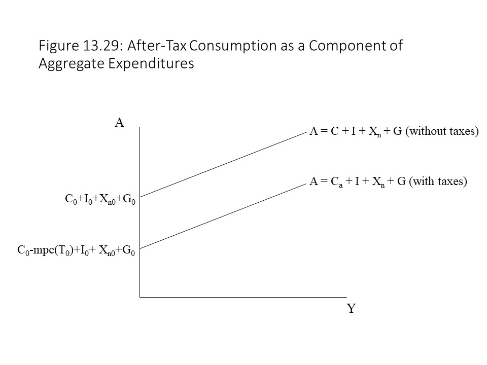 Now we can also see the impact that a lump sum tax will have on the equilibrium real GDP. When the lump sum tax is imposed, it shifts the aggregate expenditures curve down, which causes the equilibrium real GDP to fall as shown in Figure 13.30.
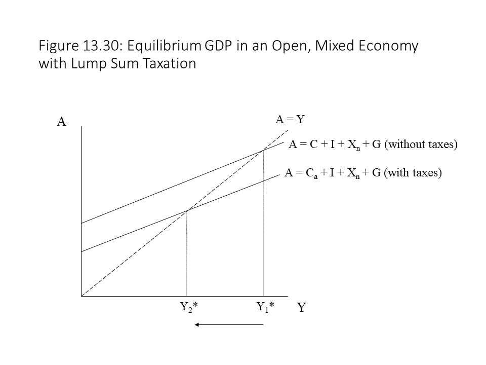 It is easy to see why a neoclassical Keynesian economist would oppose a tax increase during a recession. Higher taxes discourage consumption which reduces aggregate spending. The drop in spending leads to lower output and employment and thus harms an already weak economy. On the other hand, a tax cut can stimulate consumer spending, which will raise aggregate spending, output, and employment.
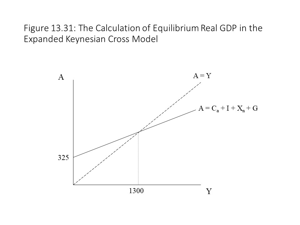
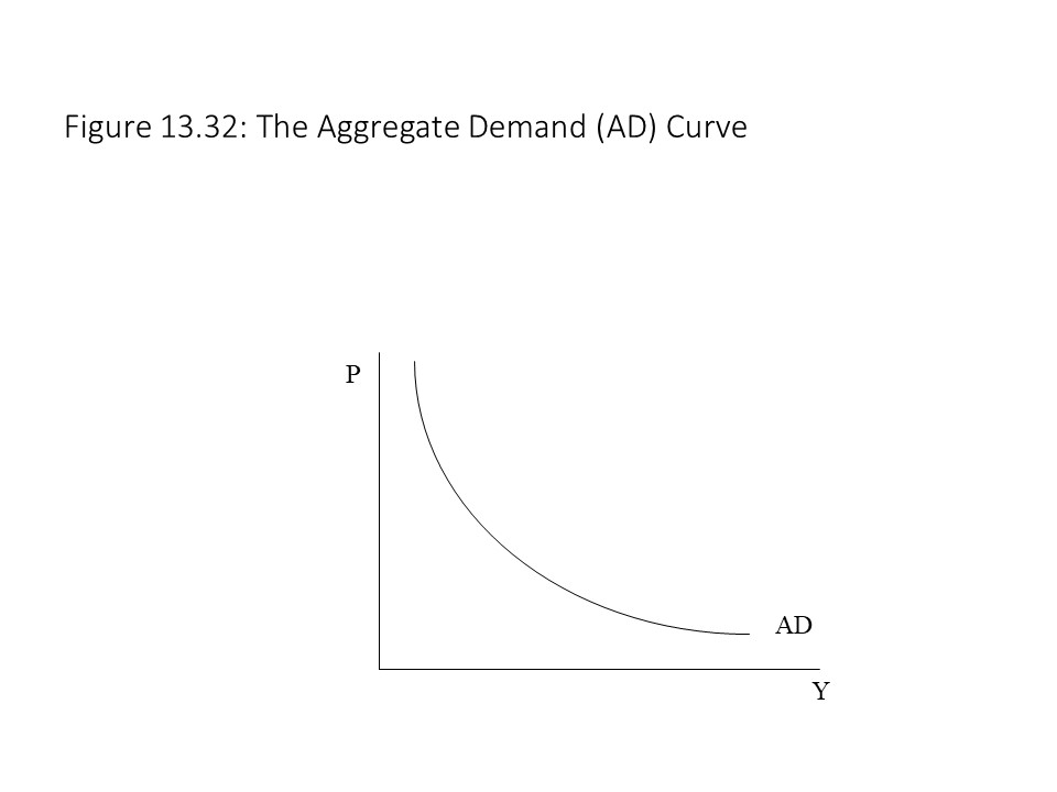 The general level of prices may be thought of as a price index such as the consumer price index or the GDP deflator. Even though the AD curve looks much like a market demand curve, it is actually quite different. It turns out that the law of demand does not apply in this context.[10] When we discussed the market demand curve in Chapter 3, it was argued that the market demand curve slopes downward for two main reasons.
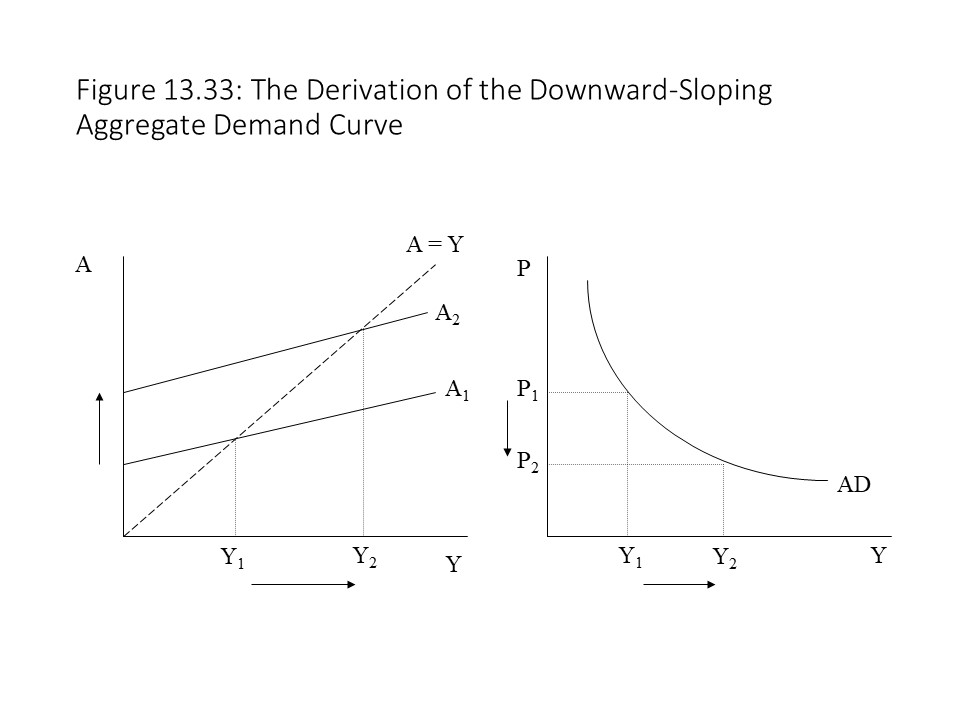
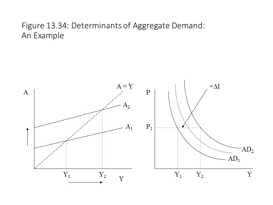
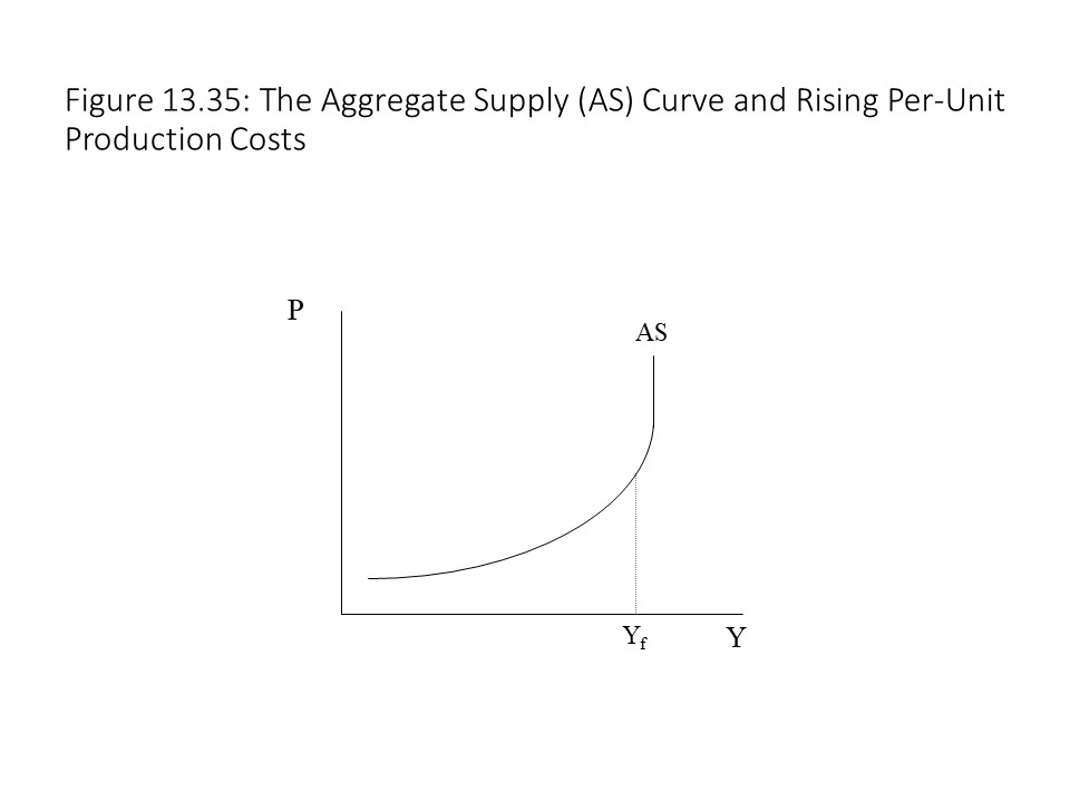
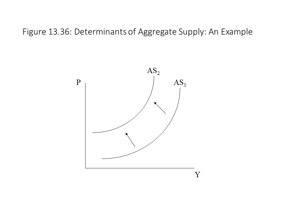 Alternatively, a reduction in the nominal wage would shift the AS curve to the right because per unit cost would be lower at every level of real GDP.
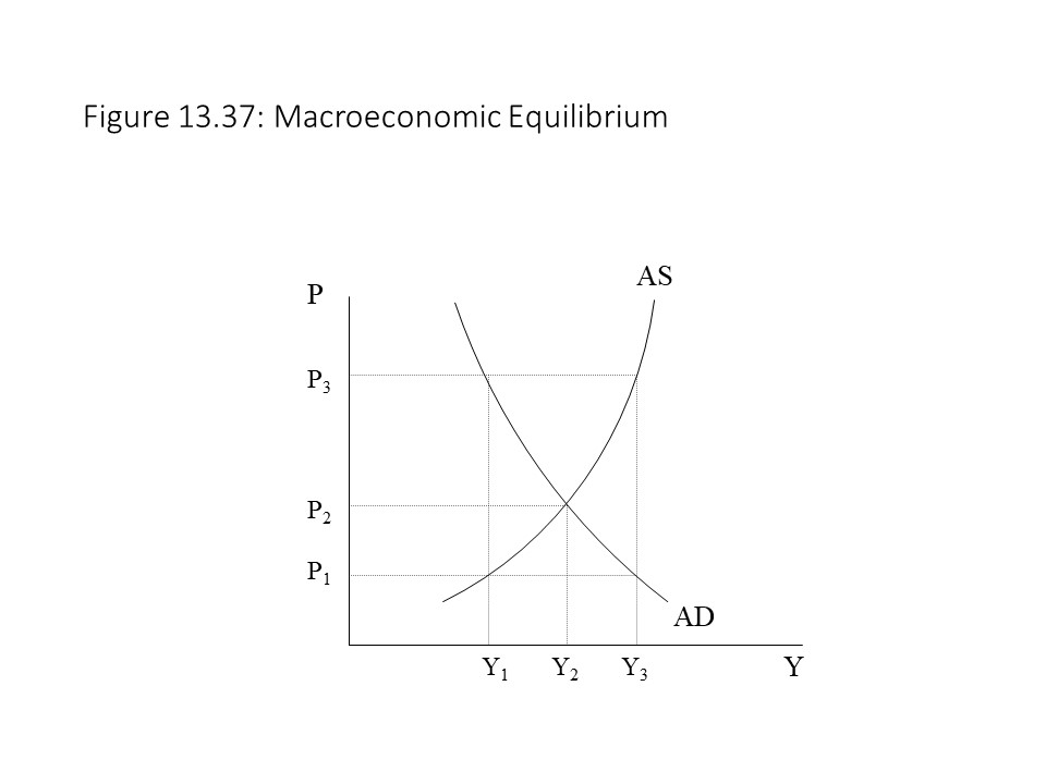
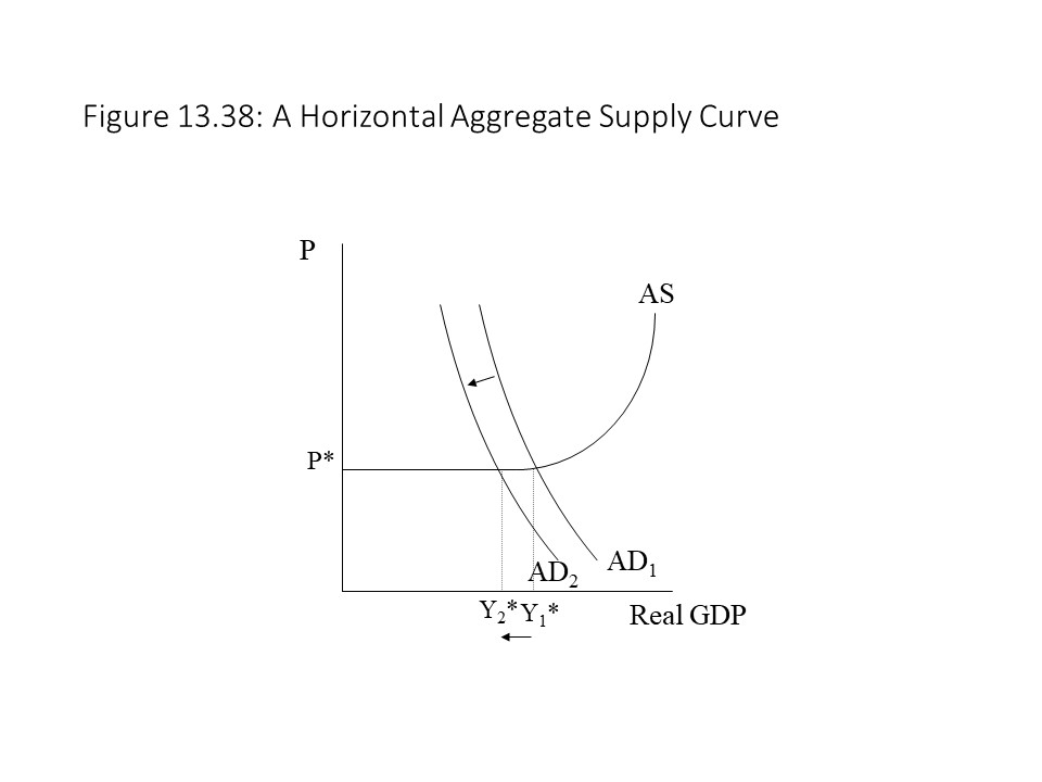 During these types of recessions, only real GDP declines. To understand why a horizontal aggregate supply curve might exist, we need to consider how conditions changed in the 1930s and 1940s. In particular, it became more difficult to reduce wages during a recession for a number of reasons, including the passage of a federal minimum wage law in 1938 and the growing power of industrial unions in major industries that negotiated high wage rates. With unit labor costs becoming more rigid, businesses could not reduce them during a recession and so they hesitated to cut prices. Other factors contributing to sticky prices might have been business concerns about menu costs (costs associated with price cuts) and efforts to avoid price wars with oligopolistic competitors.[20] The tendency for prices to be downwardly inflexible means that prices tend to increase, but once they rise, they tend not to fall again.
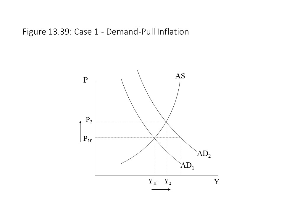
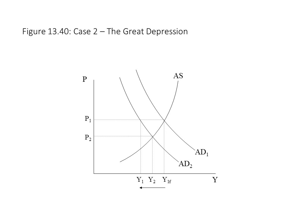 After the stock market crash of 1929, investment spending and consumer spending fell significantly. The failures of many American banks contributed significantly to the reduction in investment spending as well. As real output fell and unemployment rose, unit costs declined and the price level fell. The price level and level of real output eventually reached P2 and Y2, respectively. If the economy had been subject to downwardly inflexible prices, then the price level would have remained at P1 and the real output would have fallen to Y1. Interestingly, such price stickiness would have made the collapse of output and employment worse during the Great Depression. The falling price level actually took some of the pressure off of real output as aggregate demand fell. The reason that recessions since World War II have been less severe is not the result of sticky prices. Instead, it is because reductions in aggregate demand have been smaller as governments and central banks have become more aggressive about preventing economic collapses.
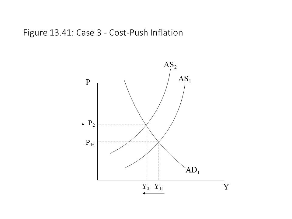
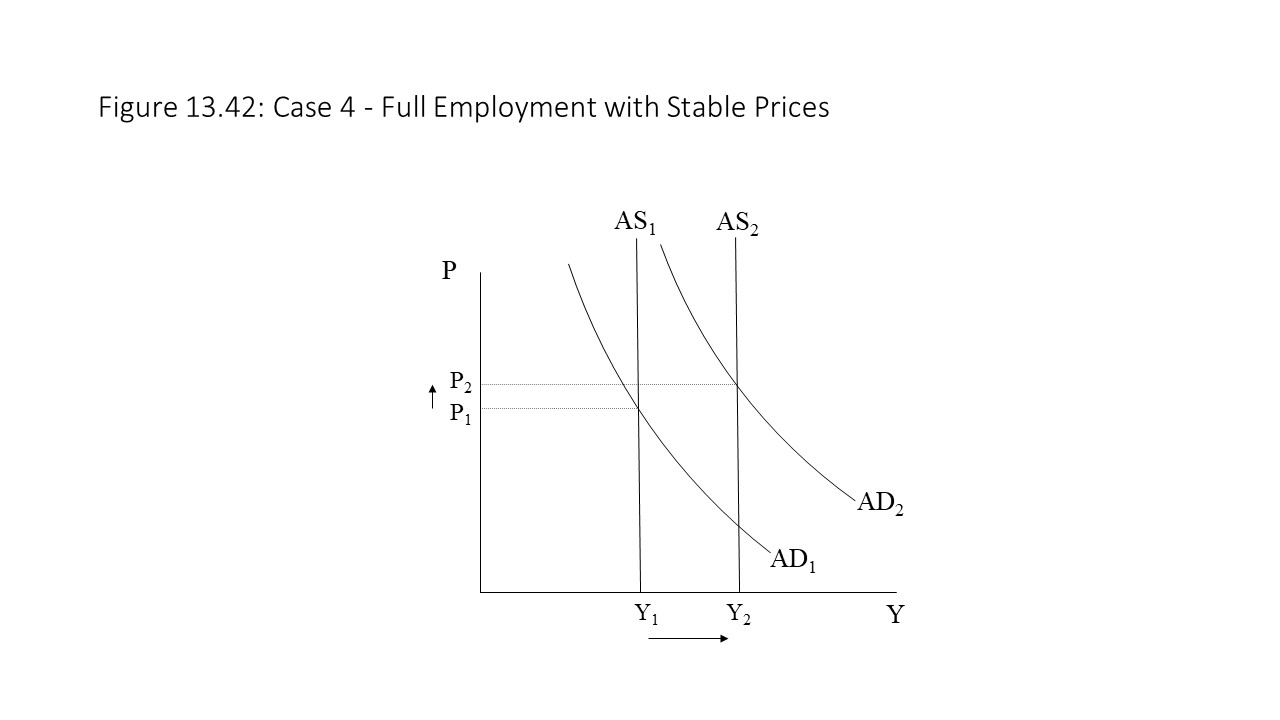
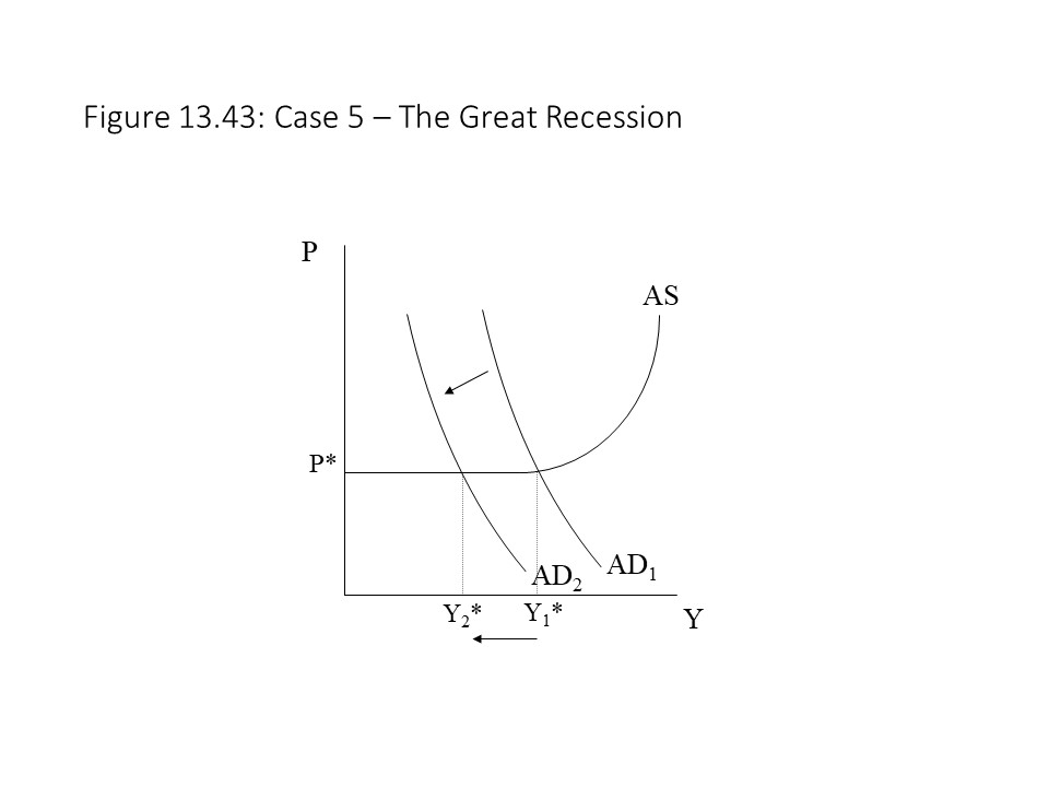 This recession was so extreme that it has been dubbed the Great Recession. It was the worst reduction in real GDP that has occurred since the Great Depression of the 1930s. It should be noted, however, that the Great Depression was far worse with a drop in real GDP and an unemployment rate in excess of 25%. By contrast, during the Great Recession, real GDP fell by just over 4% and the unemployment rate was around 10% at its peak. The reason that the Great Recession was not worse than it was stemmed from the massive government and central bank responses to the crisis. The U.S. Federal Reserve acted as a lender of last resort and offered emergency loans to large financial institutions. The federal government also passed emergency measures, including a $700 billion Troubled Asset Relief Plan (TARP) in late 2008 that bought up hundreds of billions of dollars of so-called toxic assets from banks and other financial institutions while also purchasing equity stakes in the same financial institutions. The federal government also implemented a fiscal stimulus package in early 2009 that included $787 billion of government spending increases and tax cuts. This stimulus package was consistent with the Keynesian prescription for boosting output and employment during recessions. Although these measures had some impact, economic growth remained sluggish for several years and unemployment remained stubbornly high.
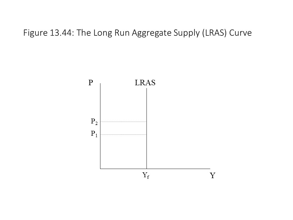 The LRAS curve is perfectly vertical. The reason is that in the long run with perfect price flexibility, all resources will be fully employed. Any unemployment in the markets for land, labor, or capital, will disappear as prices fall and eliminate the unemployment. With each factor of production fully employed, the economy will produce the full employment level of real GDP. Changes in the price level will have no impact on the level of real GDP. The only factors that can shift the LRAS curve are changes in the endowment of society’s resources (i.e., land, labor, and capital) or changes in the available production technology. Otherwise, the LRAS curve will remain where it is.
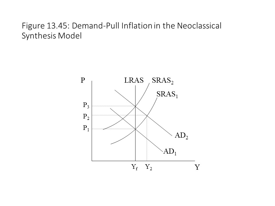 Now suppose that the central bank increases the money supply, which pushes the interest rate down and stimulates investment spending. The rise in investment spending increases aggregate demand, shifting the AD curve to the right. According to Keynesian theory, output rises above the full employment level to Y2 and the unemployment rate falls below the natural rate of unemployment. At the same time, the price level rises to P2 due to the rise in per unit cost. The Keynesian short-run explanation would stop at this point, but according to the neoclassical synthesis model, in the long run factor prices will begin to rise. As nominal wages and other factor prices rise pushing up unit cost, the SRAS curve shifts to the left. The new long run equilibrium then occurs at the intersection of AD, the new SRAS curve, and the LRAS curve. Output returns to the long run level, and the price level is permanently higher at P3. Even though Keynes’s theory provides an explanation for the short run fluctuations, the classical theory provides the long run explanation.
 4. Suppose that a lump sum tax cut of $125 is imposed on households. If the mpc is 0.82, then what will be the overall change in real GDP that results?