In order to understand test results from standardized tests it is important to be familiar with a variety of terms and concepts that are fundamental to "measurement theory", the academic study of measurement and assessment. Two major areas in measurement theory, reliability and validity, were discussed in the previous chapter; in this chapter we focus on concepts and terms associated with test scores.
The basics
Frequency distributions
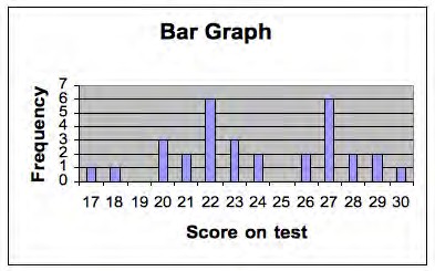
A frequency distribution is a listing of the number of students who obtained each score on a test. If 31 students take a test, and the scores range from 11 to 30 then the frequency distribution might look like Table \(\PageIndex{1}\). We also show the same set of scores on a histogram or bar graph in Exhibit \(\PageIndex{1}\). The horizontal (or x axis) represents the score on the test and the vertical axis (y axis) represents the number or frequency of students. Plotting a frequency distribution helps us see what scores are typical and how much variability there are in the scores. We describe more precise ways of determining typical scores and variability next.
Table \(\PageIndex{1}\): Frequency distribution for 30 scores
Score on test
Frequency
Central tendency measures
17
1
18
1
19
0
20
3
21
2
22
6
Mode
23
3
Median
24
2
Mean
25
0
26
2
27
6
Mode
28
2
29
2
30
1
TOTAL
31
Exhibit \(\PageIndex{1}\): Tests scores from\(\PageIndex{1}\) represented as a bar graph. (CC-BY-NC; K. Siefert, R. Sutton via Educational Psychology)
Central tendency and variability
There are three common ways of measuring central tendency or which score(s) are typical. The mean is calculated by adding up all the scores and dividing by the number of scores. In the example in Table \(\PageIndex{1}\), the mean is 24. The median is the "middle" score of the distribution— that is half of the scores are above the median and half are below. The median on the distribution is 23 because 15 scores are above 23 and 15 are below. The mode is the score that occurs most often. In Table \(\PageIndex{1}\) there are actually two modes 22 and 27 and so this distribution is described as bimodal. Calculating the mean, median and mode are important as each provides different information for teachers. The median represents the score of the "middle" students, with half scoring above and below, but does not tell us about the scores on the test that occurred most often. The mean is important for some statistical calculations but is highly influenced by a few extreme scores (called outliers) but the median is not. To illustrate this, imagine a test out of 20 points taken by 10 students, and most do very well but one student does very poorly. The scores might be 4, 18, 18, 19, 19, 19, 19, 19, 20, 20. The mean is 17.5 (170/10) but if the lowest score (4) is eliminated the mean is now is 1.5 points higher at 19 (171/9). However, in this example the median remains at 19 whether the lowest score is included. When there are some extreme scores the median is often more useful for teachers in indicating the central tendency of the frequency distribution.
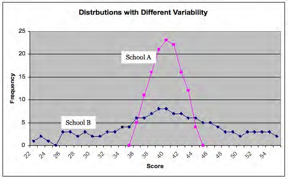
The measures of central tendency help us summarize scores that are representative, but they do not tell us anything about how variable or how spread out are the scores. Exhibit \(\PageIndex{2}\) illustrates sets of scores from two different schools on the same test for fourth graders. Note that the mean for each is 40 but in School A the scores are much less spread out. A simple way to summarize variability is the range, which is the lowest score subtracted from the lowest score. In School A with low variability the range is (45—35) = 10; in the school B the range is ( 55- 22 = 33).
Exhibit \(\PageIndex{2}\): Fourth grade math scores in two different schools with the same mean but different variability. (CC-BY-NC; K. Siefert, R. Sutton via Educational Psychology)
However, the range is only based on two scores in the distribution, the highest and lowest scores, and so does not represent variability in all the scores. The standard deviation is based on how much, on average, all the scores deviate from the mean. In the example in Exhibit 17 the standard deviations are 7.73 for School A and 2.01 for School B. In the exercise below we demonstrate how to calculate the standard deviation.
Calculating a standard deviation
Example: The scores from 11 students on a quiz are 4, 7, 6, 3, 10, 7, 3, 7, 5, 5, and 9
Order scores.
Calculate the mean score.
Calculate the deviations from the mean.
Square the deviations from the mean.
Calculate the mean of the squared deviations from the mean (i.e. sum the squared deviations from the mean then divide by the number of scores). This number is called the variance.
Take the square root and you have calculated the standard deviation.
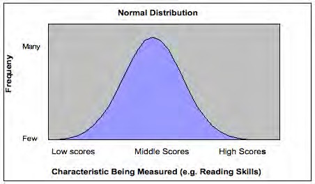
Knowing the standard deviation is particularly important when the distribution of the scores falls on a normal distribution. When a standardized test is administered to a very large number of students the distribution of scores is typically similar, with many students scoring close to the mean, and fewer scoring much higher or lower than the mean. When the distribution of scores looks like the bell shape shown in Exhibit \(\PageIndex{2}\) it is called a normal distribution. In the diagram we did not draw in the scores of individual students as we did in Exhibit \(\PageIndex{1}\), because distributions typically only fall on a normal curve when there are a large number of students; too many to show individually. A normal distribution is symmetric, and the mean, median and mode are all the same.
Figure \(\PageIndex{3}\): Bell shaped curve of normal distribution. (CC-BY-NC; K. Siefert, R. Sutton via Educational Psychology)
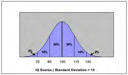
Normal curve distributions are very important in education and psychology because of the relationship between the mean, standard deviation, and percentiles. In all normal distributions 34 per cent of the scores fall between the mean and one standard deviation of the mean. Intelligence tests often are constructed to have a mean of 100 and standard deviation of 15 and we illustrate that in Exhibit \(\PageIndex{4}\).
Figure \(\PageIndex{4}\): Normal distribution for an IQ test with mean 100 and standard deviation 15. (CC-BY-NC; K. Siefert, R. Sutton via Educational Psychology)
In this example, 34 per cent of the scores are between 100 and 115 and as well, 34 per cent of the scores lie between 85 and 100. This means that 68 per cent of the scores are between -1 and +1 standard deviations of the mean (i.e. 85 and 115). Note than only 14 per cent of the scores are between +1 and +2 standard deviations of the mean and only 2 per cent fall above +2 standard deviations of the mean.
In a normal distribution a student who scores the mean value is always in the fiftieth percentile because the mean and median are the same. A score of +1 standard deviation above the mean (e.g. 115 in the example above) is the 84 per cent tile (50 per cent and 34 per cent of the scores were below 115). In Exhibit 14.2.1 we represented the percentile equivalents to the normal curve and we also showed standard scores.
Kinds of test scores
A standard score expresses performance on a test in terms of standard deviation units above of below the mean (Linn & Miller, 2005). There are a variety of standard scores:
Z-score: One type of standard score is a z-score, in which the mean is o and the standard deviation is 1. This means that a z-score tells us directly how many standard deviations the score is above or below the mean. For example, if a student receives a z score of 2 her score is two standard deviations above the mean or the eighty- fourth percentile. A student receiving a z score of -1.5 scored one and one half deviations below the mean. Any score from a normal distribution can be converted to a z score if the mean and standard deviation is known. The formula is:
So, if the score is 130 and the mean is 100 and the standard deviation is 15 then the calculation is
\[ Z_{score} = \dfrac{130-100}{15}\]
If you look at Exhibit 15 you can see that this is correct— a score of 130 is 2 standard deviations above the mean and so the z score is 2.
T-score: A T-score has a mean of 50 and a standard deviation of 10. This means that a T-score of 70 is two standard deviations above the mean and so is equivalent to a z-score of 2.
Stanines: Stanines (pronounced staynines) are often used for reporting students' scores and are based on a standard nine point scale and with a mean of 5 and a standard deviation of 2. They are only reported as whole numbers and Figure 11-10 shows their relation to the normal curve.
Grade equivalent sores
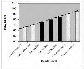
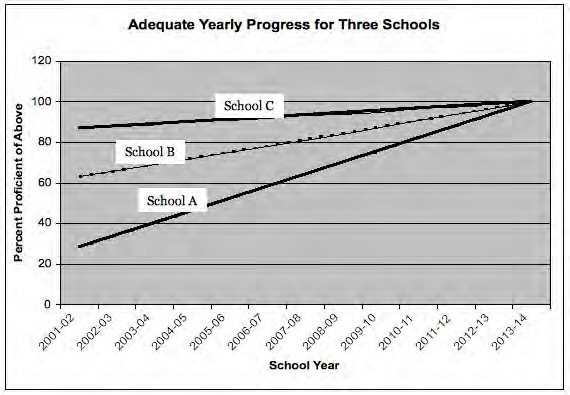
A grade equivalent score provides an estimate of test performance based on grade level and months of the school year (Popham, 2005, p. 288). A grade equivalent score of 3.7 means the performance is at that expected of a third grade student in the seventh month of the school year. Grade equivalents provide a continuing range of grade levels and so can be considered developmental scores. Grade equivalent scores are popular and seem easy to understand however they are typically misunderstood. If, James, a fourth grade student, takes a reading test and the grade equivalent score is 6.0; this does not mean that James can do sixth grade work. It means that James performed on the fourth grade test as a sixth grade student is expected to perform. Testing companies calculate grade equivalents by giving one test to several grade levels. For example a test designed for fourth graders would also be given to third and fifth graders. The raw scores are plotted and a trend line is established and this is used to establish the grade equivalents.
Figure \(\PageIndex{5}\): Using trend lines to estimate grade equivalent scores. (CC-BY-NC; K. Siefert, R. Sutton via Educational Psychology)
Grade equivalent scores also assume that the subject matter that is being tested is emphasized at each grade level to the same amount and that mastery of the content accumulates at a mostly constant rate (Popham, 2005). Many testing experts warn that grade equivalent scores should be interpreted with considerable skepticism and that parents often have serious misconceptions about grade equivalent scores. Parents of high achieving students may have an inflated sense of what their child's levels of achievement.

