8.5: Natural Constraints

Some researchers would argue that perception is a form of cognition, because it uses inferential reasoning or problem solving processing to go beyond the information given. However, this kind of account is not the only viable approach for dealing with the poverty of the visual stimulus. Rock (1983, p. 3) wrote: “A phenomenon may appear to be intelligent, but the mechanism underlying it may have no common ground with the mechanisms underlying reasoning, logical thought, or problem solving.” The natural computation approach to vision (Ballard, 1997; Marr, 1982; Richards, 1988) illustrates the wisdom of Rock’s quote, because it attempts to solve problems of underdetermination by using bottom-up devices that apply built-in constraints to filter out incorrect interpretations of an ambiguous proximal stimulus.

The central idea underlying natural computation is constraint propagation. Imagine a set of locations to which labels can be assigned, where each label is a possible property that is present at a location. Underdetermination exists when more than one label is possible at various locations. However, constraints can be applied to remove these ambiguities. Imagine that if some label x is assigned to one location then this prevents some other label y from being assigned to a neighbouring location. Say that there is good evidence to assign label x to the first location. Once this is done, a constraint can propagate outwards from this location to its neighbours, removing label y as a possibility for them and therefore reducing ambiguity.

Constraint propagation is part of the science underlying the popular Sudoku puzzles (Delahaye, 2006). A Sudoku puzzle is a 9 × 9 grid of cells, as illustrated in Figure 8-3. The grid is further divided into a 3 × 3 array of smaller 3 × 3 grids called cages. In Figure 8-3, the cages are outlined by the thicker lines. When the puzzle is solved, each cell will contain a digit from the range 1 to 9, subject to three constraints. First, a digit can occur only once in each row of 9 cells across the grid. Second, a digit can only occur once in each column of 9 cells along the grid. Third, a digit can only occur once in each cage in the grid. The puzzle begins with certain numbers already assigned to their cells, as illustrated in Figure 8-3. The task is to fill in the remaining digits in such a way that none of the three constraining rules are violated.

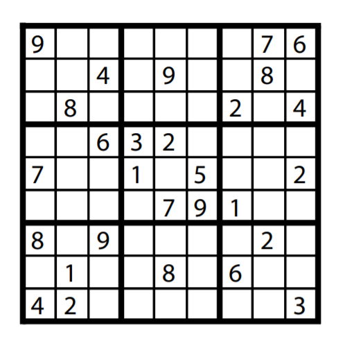
Figure 8-3. An example Sudoku puzzle.

A Sudoku puzzle can be considered as a problem to be solved by relaxation labelling. In relaxation labelling, sets of possible labels are available at different locations. For instance, at the start of the puzzle given in Figure 8-3 the possible labels at every blank cell are 1, 2, 3, 4, 5, 6, 7, 8, and 9. There is only one possible label (given in the figure) that has already been assigned to each of the remaining cells. The task of relaxation labelling is to iteratively eliminate extra labels at the ambiguous locations, so that at the end of processing only one label remains.

Figure 8-4. The “there can be only one” constraint propagating from the cell labelled 5

In the context of relaxation labelling, Sudoku puzzles can be solved by propagating different constraints through the grid; this causes potential labels to be removed from ambiguous cells. One key constraint, called “there can be only one,” emerges from the primary definition of a Sudoku puzzle. In the example problem given in Figure 8-3, the digit 5 has been assigned at the start to a particular location, which is also shown in Figure 8-4. According to the rules of Sudoku, this means that this digit cannot appear anywhere else in the column, row, or cage that contains this location. The affected locations are shaded dark grey in Figure 8-4. One can propagate the “there can be only one” constraint through these locations, removing the digit 5 as a possible label for any of them.

This constraint can be propagated iteratively through the puzzle. During one iteration, any cell with a unique label can be used to eliminate that label from all of the other cells that it controls (e.g., as in Figure 8-4). When this constraint is applied in this way, the result may be that some new cells have unique labels. In this case the constraint can be applied again, from these newly unique cells, to further disambiguate the Sudoku puzzle.

The “there can be only one” constraint is important, but it is not powerful enough on its own to solve any but the easiest Sudoku problems. This means that other constraints must be employed as well. Another constraint is called “last available label,” and is illustrated in Figure 8-5.

Figure 8-5A illustrates one of the cages of the Figure 8-3 Sudoku problem partway through being solved (i.e., after some iterations of “there can be only one”). The cells containing a single number have been uniquely labelled. The other cells still have more than one possible label, shown as multiple digits within the cell. Note the one cell at the bottom shaded in grey. It has the possible labels 1, 3, 5, and 9. However, this cell has the “last available label” of 9—the label 9 is not available in any other cell in the cage. Because a 9 is required to be in this cage, this means that this label must be assigned here and the cell’s other three possible labels can be removed. Note that when this is done, the “last available label” constraint applies to a second cell (shown in grey in Figure 8-5B), meaning that it can be uniquely assigned the label 1 by applying this constraint a second time.

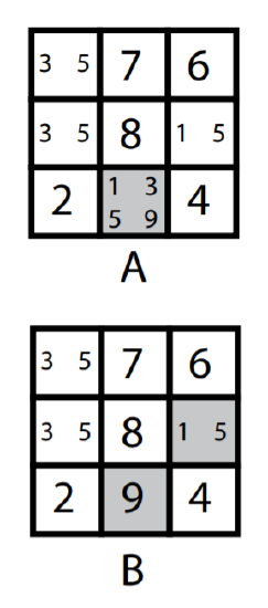
Figure 8-5. The “last available label” constraint.

After two applications of the “last available label” constraint, the cage illustrated in Figure 8-5A becomes the cage shown at the top of Figure 8-6. Note that this cage has only two ambiguous cells, each with the possible labels 3 and 5. These two cells define what Sudoku solvers call a naked pair, which can be used to define a third rule called the “naked pair constraint.”

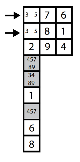
Figure 8-6. The “naked pair constraint.”

In the naked pair pointed out by the two arrows in Figure 8-6, it is impossible for one cell to receive the label 3 and for the other cell not to receive the label 5. This is because these two cells have only two remaining possible labels, and both sets of labels are identical. However, this also implies that the labels 3 and 5 cannot exist elsewhere in the part of the puzzle over which the two cells containing the naked pair have control. Thus one can use this as a constraint to remove the possible labels 3 and 5 from the other cells in the same column as the naked pair, i.e., the cells shaded in grey in the lower part of Figure 8-6.

The three constraints described above have been implemented as a working model in an Excel spreadsheet. This model has confirmed that by applying only these three constraints one can solve a variety of Sudoku problems of easy and medium difficulty, and can make substantial progress on difficult problems. (These three constraints are not sufficient to solve the difficult Figure 8-3 problem.) In order to develop a more successful Sudoku solver in this framework, one would have to identify additional constraints that can be used. A search of the Internet for “Sudoku tips” reveals a number of advanced strategies that can be described as constraints, and which could be added to a relaxation labelling model.

For our purposes, though, the above Sudoku example illustrates how constraints can be propagated to solve problems of underdetermination. Furthermore, it shows that such solutions can be fairly mechanical in nature, not requiring higher-order reasoning or problem solving. For instance, the “there can be only one” constraint could be instantiated as a simple set of interconnected switches: turning the 5 on in Figure 8-4 would send a signal that would turn the 5 off at all of the other greyshaded locations.

The natural computation approach to vision assumes that problems of visual underdetermination are also solved by non-cognitive processes that use constraint propagation. However, the constraints of interest to such researchers are not formal rules of a game. Instead, they adopt naïve realism, and they assume that the external world is structured and that some aspects of this structure must be true of nearly every visual scene. Because the visual system has evolved to function in this structured environment, it has internalized those properties that permit it to solve problems of underdetermination. “The perceptual system has internalized the most pervasive and enduring regularities of the world” (Shepard, 1990, p. 181).

The regularities of interest to researchers who endorse natural computation are called natural constraints. A natural constraint is a property that is almost invariably true of any location in a visual scene. For instance, many visual properties of threedimensional scenes, such as depth, colour, texture, and motion, vary smoothly. This means that two locations in the three-dimensional scene that are very close together are likely to have very similar values for any of these properties, while this will not be the case for locations that are further apart. Smoothness can therefore be used to constrain interpretations of a proximal stimulus: an interpretation whose properties vary smoothly is much more likely to be true of the world than interpretations in which property smoothness is not maintained.

Natural constraints are used to solve visual problems of underdetermination by imposing additional restrictions on scene interpretations. In addition to being consistent with the proximal stimulus, the interpretation of visual input must also be consistent with the natural constraints. With appropriate natural constraints, only a single interpretation will meet both of these criteria (for many examples, see Marr, 1982). A major research goal for those who endorse the natural computation approach to vision is identifying natural constraints that filter out correct interpretations from all the other (incorrect) possibilities.

For example, consider the motion correspondence problem (Ullman, 1979), which is central to Pylyshyn’s (2003b, 2007) hybrid theory of visual cognition. In the motion correspondence problem, a set of elements is seen at one time, and another set of elements is seen at a later time. In order for the visual system to associate a sense of movement to these elements, their identities must be tracked over time. The assertion that some element x, seen at time t, is the “same thing” as some other element y, seen at time t + 1, is called a motion correspondence match. However, the assignment of motion correspondence matches is underdetermined. This is illustrated in Figure 8-7 as a simple apparent motion stimulus in which two squares (dashed outlines) are presented at one time, and then later presented in different locations (solid outlines). For this display there are two logical sets of motion correspondence matches that can be assigned, shown in B and C of the figure. Both sets of matches are consistent with the display, but they represent radically different interpretations of the identities of the elements over time. Human observers of this display will invariably experience it as Figure 8-7B, and never as Figure 8-7C. Why is this interpretation preferred over the other one, which seems just as logically plausible?

The natural computation approach answers this question by claiming that the interpretation illustrated in Figure 8-7B is consistent with additional natural constraints, while the interpretation in Figure 8-7C is not. A number of different natural constraints on the motion correspondence problem have been identified and then incorporated into computer simulations of motion perception (Dawson, 1987, 1991; Dawson, Nevin-Meadows,&Wright, 1994; Dawson&Pylyshyn, 1988; Dawson& Wright, 1989, 1994; Ullman, 1979).

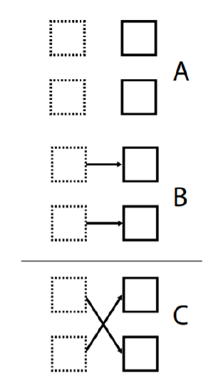
Figure 8-7. The motion correspondence problem.

One such constraint is called the nearest neighbour principle. The visual system prefers to assign correspondence matches that represent short element displacements (Burt & Sperling, 1981; Ullman, 1979). For example, the two motion correspondence matches in Figure 8-7B are shorter than the two in Figure 8-7C; they are therefore more consistent with the nearest neighbour principle.

The nearest neighbour principle is a natural constraint because it arises from the geometry of the typical viewing conditions for motion (Ullman, 1979, pp. 114–118). When movement in a three-dimensional world is projected onto a two-dimensional surface (e.g., the retina), slower movements occur with much higher probability on the retina than do faster movements. A preference for slower movement is equivalent to exploiting the nearest neighbour principle, because a short correspondence match represents slow motion, while a long correspondence match represents fast motion.

Another powerful constraint on the motion correspondence problem is called the relative velocity principle (Dawson, 1987, 1991). To the extent that visual elements arise from physical features on solid surfaces, the movement of neighbouring elements should be similar. According to the relative velocity principle, motion correspondence matches should be assigned in such a way that objects located near one another will be assigned correspondence matches consistent with movements of similar direction and speed. This is true of the two matches illustrated in Figure 8-7B, which are of identical length and direction, but not of the two matches illustrated in Figure 8-7C, which are of identical length but represent motion in different directions.

Like the nearest neighbour constraint, the relative velocity principle is a natural constraint. It is a variant of the property that motion varies smoothly across a scene (Hildreth, 1983; Horn & Schunk, 1981). That is, as objects in the real world move, locations near to one another should move in similar ways. Furthermore, Hildreth (1983) has proven that solid objects moving arbitrarily in three-dimensional space project unique smooth patterns of retinal movement. The relative velocity principle exploits this general property of projected motion.

Other natural constraints on motion correspondence have also been proposed. The element integrity principle is a constraint in which motion correspondence matches are assigned in such a way that elements only rarely split into two or fuse together into one (Ullman, 1979). It is a natural constraint in the sense that the physical coherence of surfaces implies that the splits or fusions are unlikely. The polarity matching principle is a constraint in which motion correspondence matches are assigned between elements of identical contrast (e.g., between two elements that are both light against a dark background, or between two elements that are both dark against a light background) (Dawson, Nevin-Meadows, & Wright, 1994). It is a natural constraint because movement of an object in the world might change its shape and colour, but is unlikely to alter the object’s contrast relative to its background.

The natural computation approach to vision is an alternative to a classical approach called unconscious inference, because natural constraints can be exploited by systems that are not cognitive, that do not perform inferences on the basis of cognitive contents. In particular, it is very common to see natural computation models expressed in a very anti-classical form, namely, artificial neural networks (Marr, 1982). Indeed, artificial neural networks provide an ideal medium for propagating constraints to solve problems of underdetermination.

The motion correspondence problem provides one example of an artificial neural network approach to solving problems of underdetermination (Dawson, 1991; Dawson, Nevin-Meadows, &Wright, 1994). Dawson (1991) created an artificial neural network that incorporated the nearest neighbour, relative velocity, element integrity, and polarity matching principles. These principles were realized as patterns of excitatory and inhibitory connections between processors, with each processor representing a possible motion correspondence match. For instance, the connection between two matches that represented movements similar in distance and direction would have an excitatory component that reflected the relative velocity principle. Two matches that represented movements of different distances and directions would have an inhibitory component that reflected the same principle. The network would start with all processors turned on to similar values (indicating that each match was initially equally likely), and then the network would iteratively send signals amongst the processors. The network would quickly converge to a state in which some processors remained on (representing the preferred correspondence matches) while all of the others were turned off. This model was shown to be capable of modelling a wide variety of phenomena in the extensive literature on the perception of apparent movement.

The natural computation approach is defined by another characteristic that distinguishes it from classical cognitive science. Natural constraints are not psychological properties, but are instead properties of the world, or properties of how the world projects itself onto the eyes. “The visual constraints that have been discovered so far are based almost entirely on principles that derive from laws of optics and projective geometry” (Pylyshyn, 2003b, p. 120). Agents exploit natural constraints—or more precisely, they internalize these constraints in special processors that constitute what Pylyshyn calls early vision—because they are generally true of the world and therefore work.

To classical theories that appeal to unconscious inference, natural constraints are merely “heuristic bags of tricks” that happen to work (Anstis, 1980; Ramachandran & Anstis, 1986); there is no attempt to ground these tricks in the structure of the world. In contrast, natural computation theories are embodied, because they appeal to structure in the external world and to how that structure impinges on perceptual agents. As naturalist Harold Horwood (1987, p. 35) writes, “If you look attentively at a fish you can see that the water has shaped it. The fish is not merely in the water: the qualities of the water itself have called the fish into being.