4.12: Trigger Features

For more than half a century, neuroscientists have studied vision by mapping the receptive fields of individual neurons (Hubel & Wiesel, 1959; Lettvin, Maturana, McCulloch, & Pitts, 1959). To do this, they use a method called microelectrode recording or wiretapping (Calvin & Ojemann, 1994), in which the responses of single neurons are measured while stimuli are being presented to an animal. With this technique, it is possible to describe a neuron as being sensitive to a trigger feature, a specific pattern that when detected produces maximum activity in the cell.

That individual neurons may be described as detecting trigger features has led some to endorse a neuron doctrine for perceptual psychology. This doctrine has the goal of discovering the trigger features for all neurons (Barlow, 1972, 1995). This is because,

a description of that activity of a single nerve cell which is transmitted to and influences other nerve cells, and of a nerve cell’s response to such influences from other cells, is a complete enough description for functional understanding of the nervous system. (Barlow, 1972, p. 380)

The validity of the neuron doctrine is a controversial issue (Bowers, 2009; Gross, 2002). Regardless, there is a possibility that identifying trigger features can help to interpret the internal workings of artificial neural networks.

For some types of hidden units, trigger features can be identified analytically, without requiring any wiretapping of hidden unit activities (Dawson, 2004). For instance, the activation function for an integration device (e.g., the logistic equation) is monotonic, which means that increases in net input always produce increases in activity. As a result, if one knows the maximum and minimum possible values for input signals, then one can define an integration device’s trigger feature simply by inspecting the connection weights that feed into it (Dawson, Kremer, & Gannon, 1994). The trigger feature is that pattern which sends the minimum signal through every inhibitory connection and the maximum signal through every excitatory connection. The monotonicity of an integration device’s activation function ensures that it will have only one trigger feature.

The notion of a trigger feature for other kinds of hidden units is more complex. Consider a value unit whose bias, m, in its Gaussian activation function is equal to 0. The trigger feature for this unit will be the feature that causes it to produce maximum activation. For this value unit, this will occur when the net input to the unit is equal to 0 (i.e., equal to the value of µ) (Dawson & Schopflocher, 1992b). The net input of a value unit is defined by a particular linear algebra operation, called the inner product, between a vector that represents a stimulus and a vector that represents the connection weights that fan into the unit (Dawson, 2004). So, when net input equals 0, this means that the inner product is equal to 0.

However, when an inner product is equal to 0, this indicates that the two vectors being combined are orthogonal to one another (that is, there is an angle of 90° between the two vectors). Geometrically speaking, then, the trigger feature for a value unit is an input pattern represented by a vector of activities that is at a right angle to the vector of connection weights.

This geometric observation raises complications, because it implies that a hidden value unit will not have a single trigger feature. This is because there are many input patterns that are orthogonal to a vector of connection weights. Any input vector that lies in the hyperplane that is perpendicular to the vector of connection weights will serve as a trigger feature for the hidden value unit (Dawson, 2004); this is illustrated in Figure \(\PageIndex{1}\).

Another consequence of the geometric account provided above is that there should be families of other input patterns that share the property of producing the same hidden unit activity, but one that is lower than the maximum activity produced by one of the trigger features. These will be patterns that all fall into the same hyperplane, but this hyperplane is not orthogonal to the vector of connection weights.

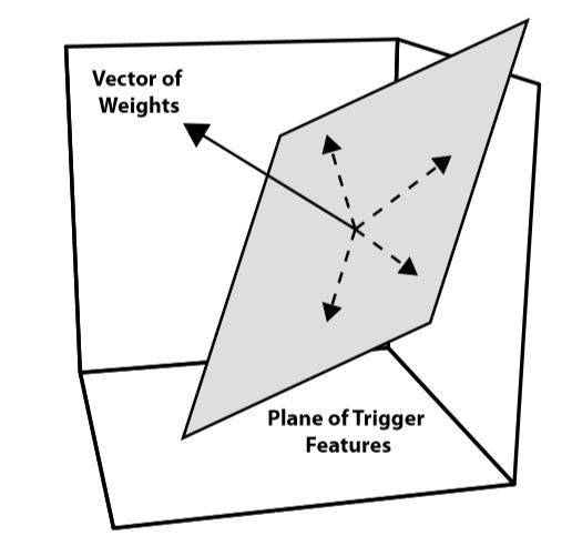Figure \(\PageIndex{1}\). Any input pattern (dashed lines) whose vector falls in the plane orthogonal to the vector of connection weights (solid line) will be a trigger feature for a hidden value unit.

The upshot of all of this is that if one trains a network of value units and then wiretaps its hidden units, the resulting hidden unit activities should be highly organized. Instead of having a rectangular distribution of activation values, there should be regular groups of activations, where each group is related to a different family of input patterns (i.e., families related to different hyperplanes of input patterns).

Empirical support for this analysis was provided by the discovery of activity banding when a hidden unit’s activities were plotted using a jittered density plot (Berkeley et al., 1995). A jittered density plot is a two-dimensional scatterplot of points; one such plot can be created for each hidden unit in a network. Each plotted point represents one of the patterns presented to the hidden unit during wiretapping. The \(x\)-value of the point’s position in the graph is the activity produced in that hidden unit by the pattern. The \(y\)-value of the point’s position in the scatterplot is a random value that is assigned to reduce overlap between points.

An example of a jittered density plot for a hidden value unit is provided in Figure \(\PageIndex{2}\). Note that the points in this plot are organized into distinct bands, which is consistent with the geometric analysis. This particular unit belongs to a network of value units trained on a logic problem discussed in slightly more detail below (Bechtel & Abrahamsen, 1991), and was part of a study that examined some of the implications of activity banding (Dawson & Piercey, 2001).

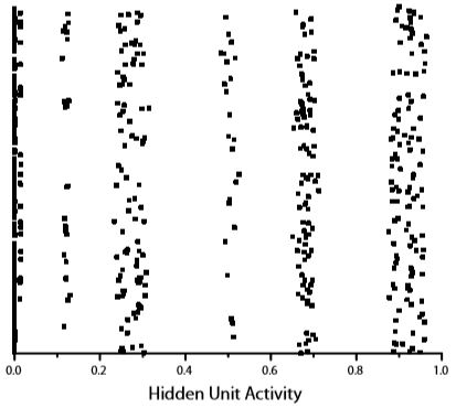
Figure \(\PageIndex{2}\). An example of banding in a jittered density plot of a hidden value unit in a network that was trained on a logic problem.

Bands in jittered density plots of hidden value units can be used to reveal the kinds of features that are being detected by these units. For instance, Berkeley et al. (1995) reported that all of the patterns that fell into the same band on a single jittered density plot in the networks did so because they shared certain local properties or features, which are called definite features.

There are two types of definite features. The first is called a definite unary feature. When a definite unary feature exists, it means that a single feature has the same value for every pattern in the band. The second is called a definite binary feature. With this kind of definite feature, an individual feature is not constant within a band. However, its relationship to some other feature is constant—variations in one feature are perfectly correlated with variations in another. Berkeley et al. (1995) showed how definite features could be both objectively defined and easily discovered using simple descriptive statistics (see also Dawson, 2005).

Definite features are always expressed in terms of the values of input unit activities. As a result, they can be assigned meanings using knowledge of a network’s input unit encoding scheme.

One example of using this approach was presented in Berkeley et al.’s (1995) analysis of a network on the Bechtel and Abrahamsen (1991) logic task. This task consists of a set of 576 logical syllogisms, each of which can be expressed as a pattern of binary activities using 14 input units. Each problem is represented as a first sentence that uses two variables, a connective or a second sentence that states a variable, and a conclusion that states a variable. Four different problem types were created in this format: modus ponens, modus tollens, disjunctive syllogism, and alternative syllogism. Each problem type was created using one of three different connectives and four different variables: the connectives were If…then, Or, or Not Both… And; the variables were A, B, C, and D. An example of a valid modus ponens argument in this format is “Sentence 1: ‘If A then B’; Sentence 2: ‘A’; Conclusion: ‘B’.”

For this problem, a network’s task is to classify an input problem into one of the four types and to classify it as being either a valid or an invalid example of that problem type. Berkeley et al. (1995) successfully trained a network of value units that employed 10 hidden units. After training, each of these units were wiretapped using the entire training set as stimulus patterns, and a jittered density plot was produced for each hidden unit. All but one of these plots revealed distinct banding. Berkeley et al. were able to provide a very detailed set of definite features for each of the bands.

After assigning definite features, Berkeley et al. (1995) used them to explore how the internal structure of the network was responsible for making the correct logical judgments. They expressed input logic problems in terms of which band of activity they belonged to for each jittered density plot. They then described each pattern as the combination of definite features from each of these bands, and they found that the internal structure of the network represented rules that were very classical in nature.

For example, Berkeley et al. (1995) found that every valid modus ponens problem was represented as the following features: having the connective If…then, having the first variable in Sentence 1 identical to Sentence 2, and having the second variable in Sentence 1 identical to the Conclusion. This is essentially the rule for valid modus ponens that could be taught in an introductory logic class (Bergmann, Moor, & Nelson, 1990). Berkeley et al. found several such rules; they also found a number that were not so traditional, but which could still be expressed in a classical form. This result suggests that artificial neural networks might be more symbolic in nature than connectionist cognitive scientists care to admit (Dawson, Medler, & Berkeley, 1997).

Importantly, the Berkeley et al. (1995) analysis was successful because the definite features that they identified were local. That is, by examining a single band in a single jittered density plot, one could determine a semantically interpretable set of features. However, activity bands are not always local. In some instances hidden value units produce nicely banded jittered density plots that possess definite features, but these features are difficult to interpret semantically (Dawson & Piercey, 2001). This occurs when the semantic interpretation is itself distributed across different bands for different hidden units; an interpretation of such a network requires definite features from multiple bands to be considered in concert.

While the geometric argument provided earlier motivated a search for the existence of bands in the hidden units of value unit networks, banding has been observed in networks of integration devices as well (Berkeley & Gunay, 2004). That being said, banding is not seen in every value unit network either. The existence of banding is likely an interaction between network architecture and problem representation; banding is useful when discovered, but it is only one tool available for network interpretation.

The important point is that practical tools exist for interpreting the internal structure of connectionist networks. Many of the technical issues concerning the relationship between classical and connectionist cognitive science may hinge upon network interpretations: “In our view, questions like ‘What is a classical rule?’ and ‘Can connectionist networks be classical in nature?’ are also hopelessly unconstrained. Detailed analysis of the internal structure of particular connectionist networks provide a specific framework in which these questions can be fruitfully pursued” (Dawson, Medler, & Berkeley, 1997, p. 39).