15.2: General Linear Model

Last updated
Save as PDF

Page ID: 26303

$ \newcommand{\vecs}[1]{\overset { \scriptstyle \rightharpoonup} {\mathbf{#1}} } $ $ \newcommand{\vecd}[1]{\overset{-\!-\!\rightharpoonup}{\vphantom{a}\smash {#1}}} $$\newcommand{\id}{\mathrm{id}}$ $ \newcommand{\Span}{\mathrm{span}}$ $ \newcommand{\kernel}{\mathrm{null}\,}$ $ \newcommand{\range}{\mathrm{range}\,}$ $ \newcommand{\RealPart}{\mathrm{Re}}$ $ \newcommand{\ImaginaryPart}{\mathrm{Im}}$ $ \newcommand{\Argument}{\mathrm{Arg}}$ $ \newcommand{\norm}[1]{\| #1 \|}$ $ \newcommand{\inner}[2]{\langle #1, #2 \rangle}$ $ \newcommand{\Span}{\mathrm{span}}$ $\newcommand{\id}{\mathrm{id}}$ $ \newcommand{\Span}{\mathrm{span}}$ $ \newcommand{\kernel}{\mathrm{null}\,}$ $ \newcommand{\range}{\mathrm{range}\,}$ $ \newcommand{\RealPart}{\mathrm{Re}}$ $ \newcommand{\ImaginaryPart}{\mathrm{Im}}$ $ \newcommand{\Argument}{\mathrm{Arg}}$ $ \newcommand{\norm}[1]{\| #1 \|}$ $ \newcommand{\inner}[2]{\langle #1, #2 \rangle}$ $ \newcommand{\Span}{\mathrm{span}}$$\newcommand{\AA}{\unicode[.8,0]{x212B}}$

Most inferential statistical procedures in social science research are derived from a general family of statistical models called the general linear model (GLM). A model is an estimated mathematical equation that can be used to represent a set of data, and linear refers to a straight line. Hence, a GLM is a system of equations that can be used to represent linear patterns of relationships in observed data.

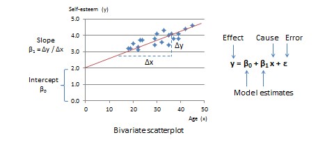
The simplest type of GLM is a two-variable linear model that examines the relationship between one independent variable (the cause or predictor) and one dependent variable (the effect or outcome). Let us assume that these two variables are age and self-esteem respectively. The bivariate scatterplot for this relationship is shown in Figure 15.1, with age (predictor) along the horizontal or -axis and self-esteem (outcome) along the vertical or -axis. From the scatterplot, it appears that individual observations representing combinations of age and self-esteem generally seem to be scattered around an upward sloping straight line. We can estimate parameters of this line, such as its slope and intercept from the GLM. From high school algebra, recall that straight lines can be represented using the mathematical equation , where is the slope of the straight line (how much does change for unit change in ?) and is the intercept term (what is the value of when is zero?). In GLM, this equation is represented formally as:

$y = \beta_{0} + \beta_{1} x + \varepsilon\,,$

where $\beta_0$ is the slope, $\beta_1$ is the intercept term, and $\varepsilon$ is the error term. $\varepsilon$ represents the deviation of actual observations from their estimated values, since most observations are close to the line but do not fall exactly on the line—i.e., the GLM is not perfect. Note that a linear model can have more than two predictors. To visualise a linear model with two predictors, imagine a three-dimensional cube, with the outcome () along the vertical axis, and the two predictors (say, and ) along the two horizontal axes at the base of the cube. A line that describes the relationship between two or more variables is called a regression line, $\beta_0$ and $\beta_1$ (and other beta values) are called regression coefficients, and the process of estimating regression coefficients is called regression analysis. The GLM for regression analysis with n predictor variables is:

$y = \beta_{0} + \beta_{1} x_{1} + \beta_{2} x_{2} + \beta_{3} x_{3} + \ldots + \beta_{n} x_{x} + \varepsilon \,.$

In the above equation, predictor variables $x_{i}$ may represent independent variables or covariates (control variables). Covariates are variables that are not of theoretical interest but may have some impact on the dependent variable y and should be controlled, so that the residual effects of the independent variables of interest are detected more precisely. Covariates capture systematic errors in a regression equation while the error term ( $\varepsilon$ ) captures random errors. Though most variables in the GLM tend to be interval or ratio-scaled, this does not have to be the case. Some predictor variables may even be nominal variables (e.g., gender: male or female), which are coded as dummy variables. These are variables that can assume one of only two possible values: 0 or 1 (in the gender example, ‘male’ may be designated as 0 and ‘female’ as 1 or vice versa). A set of n nominal variables is represented using dummy variables. For instance, industry sector, consisting of the agriculture, manufacturing, and service sectors, may be represented using a combination of two dummy variables $(x_{1}, x_{2})$ , with for agriculture, for manufacturing, and for service. It does not matter which level of a nominal variable is coded as 0 and which level as 1, because 0 and 1 values are treated as two distinct groups (such as treatment and control groups in an experimental design), rather than as numeric quantities, and the statistical parameters of each group are estimated separately.

The GLM is a very powerful statistical tool because it is not one single statistical method, but rather a family of methods that can be used to conduct sophisticated analysis with different types and quantities of predictor and outcome variables. If we have a dummy predictor variable, and we are comparing the effects of the two levels—0 and 1—of this dummy variable on the outcome variable, we are doing an analysis of variance (ANOVA). If we are doing ANOVA while controlling for the effects of one or more covariates, we have an analysis of covariance (ANCOVA). We can also have multiple outcome variables—e.g., $y_{1}$ , $y_{2}$ , $\ldots$ $y_{n}$ —which are represented using a ‘system of equations’ consisting of a different equation for each outcome variable, each with its own unique set of regression coefficients. If multiple outcome variables are modelled as being predicted by the same set of predictor variables, the resulting analysis is called multivariate regression. If we are doing ANOVA or ANCOVA analysis with multiple outcome variables, the resulting analysis is a multivariate ANOVA (MANOVA) or multivariate ANCOVA (MANCOVA) respectively. If we model the outcome in one regression equation as a predictor in another equation in an interrelated system of regression equations, then we have a very sophisticated type of analysis called structural equation modelling. The most important problem in GLM is model specification—i.e., how to specify a regression equation or a system of equations—to best represent the phenomenon of interest. Model specification should be based on theoretical considerations about the phenomenon being studied, rather than what fits the observed data best. The role of data is in validating the model, and not in its specification.