The previous section discussed how to measure respondents’ responses to predesigned items or indicators belonging to an underlying construct. But how do we create the indicators themselves? The process of creating the indicators is called scaling. More formally, scaling is a branch of measurement that involves the construction of measures by associating qualitative judgments about unobservable constructs with quantitative, measurable metric units. Stevens (1946) said, “Scaling is the assignment of objects to numbers according to a rule.” This process of measuring abstract concepts in concrete terms remains one of the most difficult tasks in empirical social science research.
The outcome of a scaling process is a scale, which is an empirical structure for measuring items or indicators of a given construct. Understand that “scales”, as discussed in this section, are a little different from “rating scales” discussed in the previous section. A rating scale is used to capture the respondents’ reactions to a given item, for instance, such as a nominal scaled item captures a yes/no reaction and an interval scaled item captures a value between “strongly disagree” to “strongly agree.” Attaching a rating scale to a statement or instrument is not scaling. Rather, scaling is the formal process of developing scale items, before rating scales can be attached to those items.
Scales can be unidimensional or multidimensional, based on whether the underlying construct is unidimensional (e.g., weight, wind speed, firm size) or multidimensional (e.g., academic aptitude, intelligence). Unidimensional scale measures constructs along a single scale, ranging from high to low. Note that some of these scales may include multiple items, but all of these items attempt to measure the same underlying dimension. This is particularly the case with many social science constructs such as self-esteem, which are assumed to have a single dimension going from low to high. Multi-dimensional scales, on the other hand, employ different items or tests to measure each dimension of the construct separately, and then combine the scores on each dimension to create an overall measure of the multidimensional construct. For instance, academic aptitude can be measured using two separate tests of students’ mathematical and verbal ability, and then combining these scores to create an overall measure for academic aptitude. Since most scales employed in social science research are unidimensional, we will next three examine approaches for creating unidimensional scales.
Unidimensional scaling methods were developed during the first half of the twentieth century and were named after their creators. The three most popular unidimensional scaling methods are: (1) Thurstone’s equal-appearing scaling, (2) Likert’s summative scaling, and (3) Guttman’s cumulative scaling. The three approaches are similar in many respects, with the key differences being the rating of the scale items by judges and the statistical methods used to select the final items. Each of these methods are discussed next.
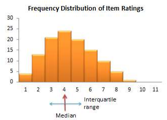
Thurstone’s equal-appearing scaling method. Louis Thurstone. one of the earliest and most famous scaling theorists, published a method of equal-appearing intervals in 1925. This method starts with a clear conceptual definition of the construct of interest. Based on this definition, potential scale items are generated to measure this construct. These items are generated by experts who know something about the construct being measured. The initial pool of candidate items (ideally 80 to 100 items) should be worded in a similar manner, for instance, by framing them as statements to which respondents may agree or disagree (and not as questions or other things). Next, a panel of judges is recruited to select specific items from this candidate pool to represent the construct of interest. Judges may include academics trained in the process of instrument construction or a random sample of respondents of interest (i.e., people who are familiar with the phenomenon). The selection process is done by having each judge independently rate each item on a scale from 1 to 11 based on how closely, in their opinion, that item reflects the intended construct (1 represents extremely unfavorable and 11 represents extremely favorable). For each item, compute the median and inter-quartile range (the difference between the 75th and the 25th percentile – a measure of dispersion), which are plotted on a histogram, as shown in Figure 6.1. The final scale items are selected as statements that are at equal intervals across a range of medians. This can be done by grouping items with a common median, and then selecting the item with the smallest inter-quartile range within each median group. However, instead of relying entirely on statistical analysis for item selection, a better strategy may be to examine the candidate items at each level and selecting the statement that is the most clear and makes the most sense. The median value of each scale item represents the weight to be used for aggregating the items into a composite scale score representing the construct of interest. We now have a scale which looks like a ruler, with one item or statement at each of the 11 points on the ruler (and weighted as such). Because items appear equally throughout the entire 11-pointrange of the scale, this technique is called an equal-appearing scale.
Thurstone also created two additional methods of building unidimensional scales – the method of successive intervals and the method of paired comparisons – which are both very similar to the method of equal-appearing intervals, except for how judges are asked to rate the data. For instance, the method of paired comparison requires each judge to make a judgment between each pair of statements (rather than rate each statement independently on a 1 to 11 scale). Hence, the name paired comparison method. With a lot of statements, this approach can be enormously time consuming and unwieldy compared to the method of equal-appearing intervals.
Figure 6.1. Histogram for Thurstone scale items
Likert’s summative scaling method. The Likert method, a unidimensional scaling method developed by Murphy and Likert (1938), is quite possibly the most popular of the three scaling approaches described in this chapter. As with Thurstone’s method, the Likert method also starts with a clear definition of the construct of interest, and using a set of experts to generate about 80 to 100 potential scale items. These items are then rated by judges on a 1 to 5 (or 1 to 7) rating scale as follows: 1 for strongly disagree with the concept, 2 for somewhat disagree with the concept, 3 for undecided, 4 for somewhat agree with the concept, and 5 for strongly agree with the concept. Following this rating, specific items can be selected for the final scale can be selected in one of several ways: (1) by computing bivariate correlations between judges rating of each item and the total item (created by summing all individual items for each respondent), and throwing out items with low (e.g., less than 0.60) item-to-total correlations, or (2) by averaging the rating for each item for the top quartile and the bottom quartile of judges, doing a t-test for the difference in means, and selecting items that have high t-values (i.e., those that discriminates best between the top and bottom quartile responses). In the end, researcher’s judgment may be used to obtain a relatively small (say 10 to 15) set of items that have high item-to-total correlations and high discrimination (i.e., high t-values). The Likert method assumes equal weights for all items, and hence, respondent’s responses to each item can be summed to create a composite score for that respondent. Hence, this method is called a summated scale. Note that any item with reversed meaning from the original direction of the construct must be reverse coded (i.e., 1 becomes a 5, 2 becomes a 4, and so forth) before summating.
Guttman’s cumulative scaling method. Designed by Guttman (1950), the cumulative scaling method is based on Emory Bogardus’ social distance technique, which assumes that people’s willingness to participate in social relations with other people vary in degrees of intensity, and measures that intensity using a list of items arranged from “least intense” to “most intense”. The idea is that people who agree with one item on this list also agree with all previous items. In practice, we seldom find a set of items that matches this cumulative pattern perfectly. A scalogram analysis is used to examine how closely a set of items corresponds to the idea of cumulativeness.
Like previous scaling methods, the Guttman method also starts with a clear definition of the construct of interest, and then using experts to develop a large set of candidate items. A group of judges then rate each candidate item as “yes” if they view the item as being favorable to the construct and “no” if they see the item as unfavorable. Next, a matrix or table is created showing the judges’ responses to all candidate items. This matrix is sorted in decreasing order from judges with more “yes” at the top to those with fewer “yes” at the bottom. Judges with the same number of “yes”, the statements can be sorted from left to right based on most number of agreements to least. The resulting matrix will resemble Table 6.6. Notice that the scale is now almost cumulative when read from left to right (across the items). However, there may be a few exceptions, as shown in Table 6.6, and hence the scale is not entirely cumulative. To determine a set of items that best approximates the cumulativeness property, a data analysis technique called scalogram analysis can be used (or this can be done visually if the number of items is small). The statistical technique also estimates a score for each item that can be used to compute a respondent’s overall score on the entire set of items.
Table 6.6. Sorted rating matrix for a Guttman scale
Respondent
Item 12
Item 5
Item 3
Item 22
Item 8
Item 7
…
29
Y
Y
Y
Y
Y
Y
7
Y
Y
Y
-
Y
-
15
Y
Y
Y
Y
-
-
3
Y
Y
Y
Y
-
-
32
Y
Y
Y
-
-
-
4
Y
Y
-
Y
-
-
5
Y
Y
-
-
-
-
23
Y
Y
-
-
-
-
11
Y
-
-
Y
-
-
Y indicates exceptions that prevents this matrix from being perfectly cumulative