In the preceding sections, we introduced terms such as population parameter, sample statistic, and sampling bias. In this section, we will try to understand what these terms mean and how they are related to each other.
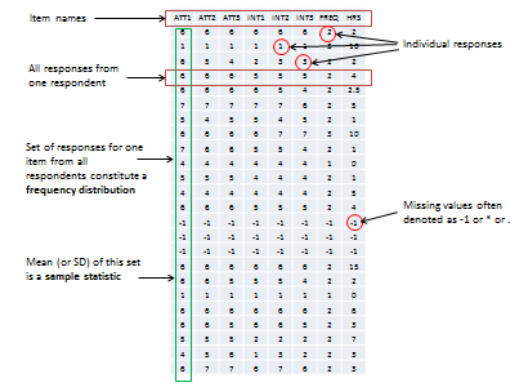
When you measure a certain observation from a given unit, such as a person’s response to a Likert-scaled item, that observation is called a response (see Figure 8.2). In other words, a response is a measurement value provided by a sampled unit. Each respondent will give you different responses to different items in an instrument. Responses from different respondents to the same item or observation can be graphed into a frequency distribution based on their frequency of occurrences. For a large number of responses in a sample, this frequency distribution tends to resemble a bell-shaped curve called a normal distribution, which can be used to estimate overall characteristics of the entire sample, such as sample mean (average of all observations in a sample) or standard deviation (variability or spread of observations in a sample). These sample estimates are called sample statistics (a “statistic” is a value that is estimated from observed data). Populations also have means and standard deviations that could be obtained if we could sample the entire population. However, since the entire population can never be sampled, population characteristics are always unknown, and are called population parameters (and not “statistic” because they are not statistically estimated from data). Sample statistics may differ from population parameters if the sample is not perfectly representative of the population; the difference between the two is called sampling error. Theoretically, if we could gradually increase the sample size so that the sample approaches closer and closer to the population, then sampling error will decrease and a sample statistic will increasingly approximate the corresponding population parameter.
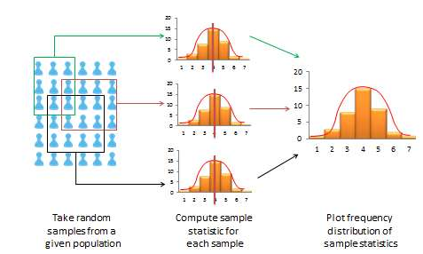
If a sample is truly representative of the population, then the estimated sample statistics should be identical to corresponding theoretical population parameters. How do we know if the sample statistics are at least reasonably close to the population parameters? Here, we need to understand the concept of a sampling distribution. Imagine that you took three different random samples from a given population, as shown in Figure 8.3, and for each sample, you derived sample statistics such as sample mean and standard deviation. If each random sample was truly representative of the population, then your three sample means from the three random samples will be identical (and equal to the population parameter), and the variability in sample means will be zero. But this is extremely unlikely, given that each random sample will likely constitute a different subset of the population, and hence, their means may be slightly different from each other. However, you can take these three sample means and plot a frequency histogram of sample means. If the number of such samples increases from three to 10 to 100, the frequency histogram becomes a sampling distribution. Hence, a sampling distribution is a frequency distribution of a sample statistic (like sample mean) from a set of samples, while the commonly referenced frequency distribution is the distribution of a response (observation) from a single sample. Just like a frequency distribution, the sampling distribution will also tend to have more sample statistics clustered around the mean (which presumably is an estimate of a population parameter), with fewer values scattered around the mean. With an infinitely large number of samples, this distribution will approach a normal distribution. The variability or spread of a sample statistic in a sampling distribution (i.e., the standard deviation of a sampling statistic) is called its standard error. In contrast, the term standard deviation is reserved for variability of an observed response from a single sample.
Figure 8.2. Sample Statistic
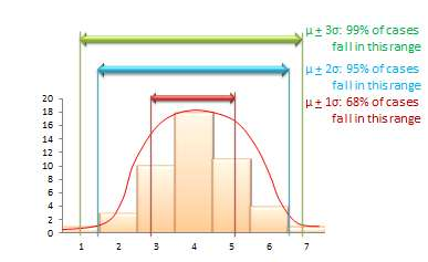
The mean value of a sample statistic in a sampling distribution is presumed to be an estimate of the unknown population parameter. Based on the spread of this sampling distribution (i.e., based on standard error), it is also possible to estimate confidence intervals for that prediction population parameter. Confidence interval is the estimated probability that a population parameter lies within a specific interval of sample statistic values. All normal distributions tend to follow a 68-95-99 percent rule (see Figure 8.4), which says that over 68% of the cases in the distribution lie within one standard deviation of the mean value (µ + 1σ), over 95% of the cases in the distribution lie within two standard deviations of the mean (µ + 2σ), and over 99% of the cases in the distribution lie within three standard deviations of the mean value (µ + 3σ). Since a sampling distribution with an infinite number of samples will approach a normal distribution, the same 68-95-99 rule applies, and it can be said that:
(Sample statistic one standard error) represents a 68% confidence interval for the population parameter.
(Sample statistic two standard errors) represents a 95% confidence interval for the population parameter.
(Sample statistic three standard errors) represents a 99% confidence interval for the population parameter.
Figure 8.3. The sampling distribution
A sample is “biased” (i.e., not representative of the population) if its sampling distribution cannot be estimated or if the sampling distribution violates the 68-95-99 percent rule. As an aside, note that in most regression analysis where we examine the significance of regression coefficients with p<0.05, we are attempting to see if the sampling statistic (regression coefficient) predicts the corresponding population parameter (true effect size) with a 95% confidence interval. Interestingly, the “six sigma” standard attempts to identify manufacturing defects outside the 99% confidence interval or six standard deviations (standard deviation is represented using the Greek letter sigma), representing significance testing at p<0.01.
Figure 8.4. The 68-95-99 percent rule for confidence interval


 one standard error) represents a 68% confidence interval for the population parameter.
 two standard errors) represents a 95% confidence interval for the population parameter.
 three standard errors) represents a 99% confidence interval for the population parameter.