

13.2.1: Critical Values of Chi-Square Table
- Page ID
- 287811

\( \newcommand{\vecs}[1]{\overset { \scriptstyle \rightharpoonup} {\mathbf{#1}} } \)
\( \newcommand{\vecd}[1]{\overset{-\!-\!\rightharpoonup}{\vphantom{a}\smash {#1}}} \)
\( \newcommand{\dsum}{\displaystyle\sum\limits} \)
\( \newcommand{\dint}{\displaystyle\int\limits} \)
\( \newcommand{\dlim}{\displaystyle\lim\limits} \)
\( \newcommand{\id}{\mathrm{id}}\) \( \newcommand{\Span}{\mathrm{span}}\)
( \newcommand{\kernel}{\mathrm{null}\,}\) \( \newcommand{\range}{\mathrm{range}\,}\)
\( \newcommand{\RealPart}{\mathrm{Re}}\) \( \newcommand{\ImaginaryPart}{\mathrm{Im}}\)
\( \newcommand{\Argument}{\mathrm{Arg}}\) \( \newcommand{\norm}[1]{\| #1 \|}\)
\( \newcommand{\inner}[2]{\langle #1, #2 \rangle}\)
\( \newcommand{\Span}{\mathrm{span}}\)
\( \newcommand{\id}{\mathrm{id}}\)
\( \newcommand{\Span}{\mathrm{span}}\)
\( \newcommand{\kernel}{\mathrm{null}\,}\)
\( \newcommand{\range}{\mathrm{range}\,}\)
\( \newcommand{\RealPart}{\mathrm{Re}}\)
\( \newcommand{\ImaginaryPart}{\mathrm{Im}}\)
\( \newcommand{\Argument}{\mathrm{Arg}}\)
\( \newcommand{\norm}[1]{\| #1 \|}\)
\( \newcommand{\inner}[2]{\langle #1, #2 \rangle}\)
\( \newcommand{\Span}{\mathrm{span}}\) \( \newcommand{\AA}{\unicode[.8,0]{x212B}}\)
\( \newcommand{\vectorA}[1]{\vec{#1}} % arrow\)
\( \newcommand{\vectorAt}[1]{\vec{\text{#1}}} % arrow\)
\( \newcommand{\vectorB}[1]{\overset { \scriptstyle \rightharpoonup} {\mathbf{#1}} } \)
\( \newcommand{\vectorC}[1]{\textbf{#1}} \)
\( \newcommand{\vectorD}[1]{\overrightarrow{#1}} \)
\( \newcommand{\vectorDt}[1]{\overrightarrow{\text{#1}}} \)
\( \newcommand{\vectE}[1]{\overset{-\!-\!\rightharpoonup}{\vphantom{a}\smash{\mathbf {#1}}}} \)
\( \newcommand{\vecs}[1]{\overset { \scriptstyle \rightharpoonup} {\mathbf{#1}} } \)
\(\newcommand{\longvect}{\overrightarrow}\)
\( \newcommand{\vecd}[1]{\overset{-\!-\!\rightharpoonup}{\vphantom{a}\smash {#1}}} \)
\(\newcommand{\ket}[1]{\left| #1 \right>}\)
\(\newcommand{\bra}[1]{\left< #1 \right|}\)
\(\newcommand{\braket}[2]{\left< #1 \vphantom{#2} \right| \left. #2 \vphantom{#1} \right>}\)
\(\newcommand{\braopket}[3]{\left< #1 \vphantom{#2}\vphantom{#3} \right| #2 \vphantom{#1}\vphantom{#3} \left| #3 \vphantom{#1}\vphantom{#2} \right>}\)
\(\newcommand{\qmvec}[1]{\mathbf{\vec{#1}}}\)
\(\newcommand{\op}[1]{\hat{\mathbf{#1}}}\)
\(\newcommand{\expect}[1]{\langle #1 \rangle}\)
\(\newcommand{\dfn}[1]{\emph{\textbf{#1}}}\)
A new type of statistical analysis, a new table of critical values!
Chi-Square Distributions
As you know, there is a whole family of \(t\)-distributions, each one specified by a parameter called the degrees of freedom (\(df\)). Similarly, all the chi-square distributions form a family, and each of its members is also specified by a its own \(df\). Chi (like "kite," not like "chai" or "Chicago") is a Greek letter denoted by the symbol \(\chi\) and chi-square is often denoted by \(\chi^2\). It looks like a wiggly X, but is not an X. Figure \(\PageIndex{1}\) shows several \(\chi\)-square distributions for different degrees of freedom.
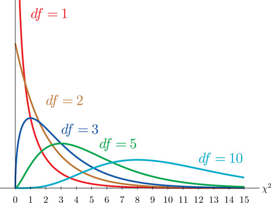 Figure \(\PageIndex{1}\): Many \(\chi\) Distributions (CC-BY-NC-SA Shafer & Zhang)
Like all tables of critical values, this one provides the value in which you should reject the null hypothesis if your calculated value is bigger than the critical value i the table. For chi-square, the null hypothesis is that there is no pattern of relationship, but the process of Null Hypothesis Signficance Testing is the same as we've been learning.
(Critical \(<\) Calculated) \(=\) Reject null \(=\) There is a pattern of relationship. \(= p<.05\)
(Critical \(>\) Calculated) \(=\) Retain null \(=\) There is no pattern of relationship. \(= p>.05\)
Illustrated in Figure \(\PageIndex{2}\), the value of the chi-square that cuts off a right tail of area \(c\) is denoted \(\chi_c^2\) and is called a critical value (Figure \(\PageIndex{2}\)).
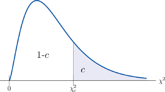 Figure \(\PageIndex{2}\): \(\chi_c^2\) Illustration of Critical Values of Chi-Square. (CC-BY-NC-SA Shafer & Zhang)
Table of Critical Values for \(\chi_c^2\)
Table \(\PageIndex{1}\) below gives values of \(\chi_c^2\) for various values of \(c\) and under several chi-square distributions with various degrees of freedom.
| df | p = 0.10 | p = 0.05 | p = 0.01 |
|---|---|---|---|
| 1 | 2.706 | 3.841 | 6.635 |
| 2 | 4.605 | 5.991 | 9.210 |
| 3 | 6.251 | 7.815 | 11.345 |
| 4 | 7.779 | 9.488 | 13.277 |
| 5 | 9.236 | 11.070 | 15.086 |
| 6 | 10.645 | 12.592 | 16.812 |
| 7 | 12.017 | 14.067 | 18.475 |
| 8 | 13.362 | 15.507 | 20.090 |
| 9 | 14.684 | 16.919 | 21.666 |
| 10 | 15.987 | 18.307 | 23.209 |
| 11 | 17.275 | 19.675 | 24.725 |
| 12 | 18.549 | 21.026 | 26.217 |
| 13 | 19.812 | 22.362 | 27.688 |
| 14 | 21.064 | 23.685 | 29.141 |
| 15 | 22.307 | 24.996 | 30.578 |
| 16 | 23.542 | 26.296 | 32.000 |
| 17 | 24.769 | 27.587 | 33.409 |
| 18 | 25.989 | 28.869 | 34.805 |
| 19 | 27.204 | 30.144 | 36.191 |
| 20 | 28.412 | 31.410 | 37.566 |
| 100 | 118.498 | 124.342 | 135.807 |
Degrees of Freedom
Like with the t-test and ANOVA, the degrees of freedom are based on which kind of analysis you are conducting.
- \(\chi_{GoF}^2\) Goodness of Fit: \(k-1\)
- k is the number of categories.
- \(\chi_{ToI}^2\) Test of Independence: \((R-1)\times(C-1) \)
- R is the number of rows
- C is the number of columns
- Kruskal-Wallis Test: \(k-1 \)
- k is the number of groups