6.3: Probability Samples

Learning Objectives

• Describe how probability sampling differs from nonprobability sampling.

• Define generalizability and describe how it is achieved in probability samples.

• Identify the various types of probability samples, and provide a brief description of each.

Quantitative researchers are often interested in being able to make generalizations about groups larger than their study samples. While there are certainly instances when quantitative researchers rely on nonprobability samples (e.g., when doing exploratory research), quantitative researchers tend to rely on probability sampling techniques. The goals and techniques associated with probability samples differ from those of nonprobability samples. We’ll explore those unique goals and techniques in this section.

Probability Sampling

Unlike nonprobability sampling, probability sampling refers to sampling techniques for which a person’s (or event’s) likelihood of being selected for membership in the sample is known. You might ask yourself why we should care about a study element’s likelihood of being selected for membership in a researcher’s sample. The reason is that, in most cases, researchers who use probability sampling techniques are aiming to identify a representative sample from which to collect data. A representative sample is one that resembles the population from which it was drawn in all the ways that are important for the research being conducted. If, for example, you wish to be able to say something about differences between men and women at the end of your study, you better make sure that your sample doesn’t contain only women. That’s a bit of an oversimplification, but the point with representativeness is that if your population varies in some way that is important to your study, your sample should contain the same sorts of variation.

Obtaining a representative sample is important in probability sampling because a key goal of studies that rely on probability samples is generalizability. In fact, generalizability is perhaps the key feature that distinguishes probability samples from nonprobability samples. Generalizability refers to the idea that a study’s results will tell us something about a group larger than the sample from which the findings were generated. In order to achieve generalizability, a core principle of probability sampling is that all elements in the researcher’s accessible population have a known chance of being selected for inclusion in the study. The important thing to remember about random selection here is that, as previously noted, it is a core principal of probability sampling. If a researcher uses random selection techniques to draw a sample, he or she will be able to estimate how closely the sample represents the larger population from which it was drawn by estimating the sampling error. Sampling error is a statistical calculation of the difference between results from a sample and the actual parameters of a population.

Types of Probability Samples

There are a variety of probability samples that researchers may use. These include simple random samples, systematic samples, stratified samples, and cluster samples.

1. Simple Random Samples

Simple random samples are the most basic type of probability sample. To draw a simple random sample, a researcher starts with a list of every single member, or element, of their accessible population of interest. This list is sometimes referred to as a sampling frame. Once that list has been created, the researcher numbers each element sequentially and then randomly selects the elements from which they will collect data. To randomly select elements, researchers use a table of numbers that have been generated randomly. Please note in this sample type every person or element has an equal chance of being selected.

There are several possible sources for obtaining a random number table. Some statistics and research methods textbooks offer such tables as appendices to the text.  A good online source is the website Stat Trek which contains a random number generator that you can use to create a random number table of whatever size you might need. Randomizer.org also offers a useful random number generator.

2. Systematic Random Samples

As you might have guessed, drawing a simple random sample can be quite tedious.  Systematic random sampling techniques are somewhat less tedious but offer the benefits of a random sample. As with simple random samples, you must be able to produce a list of every one of your population elements. Once you’ve done that, to draw a systematic sample, you’d simply select every kth element on your list. But what is k, and where on the list of population elements does one begin the selection process? k is your selection interval or the distance between the elements you select for inclusion in your study. To begin the selection process, you’ll need to figure out how many elements you wish to include in your sample. Let’s say you want to interview 25 fraternity members on your campus, and there are 100 men on campus who are members of fraternities. In this case, your selection interval, or k, is 4. To arrive at 4, simply divide the total number of population elements by your desired sample size.

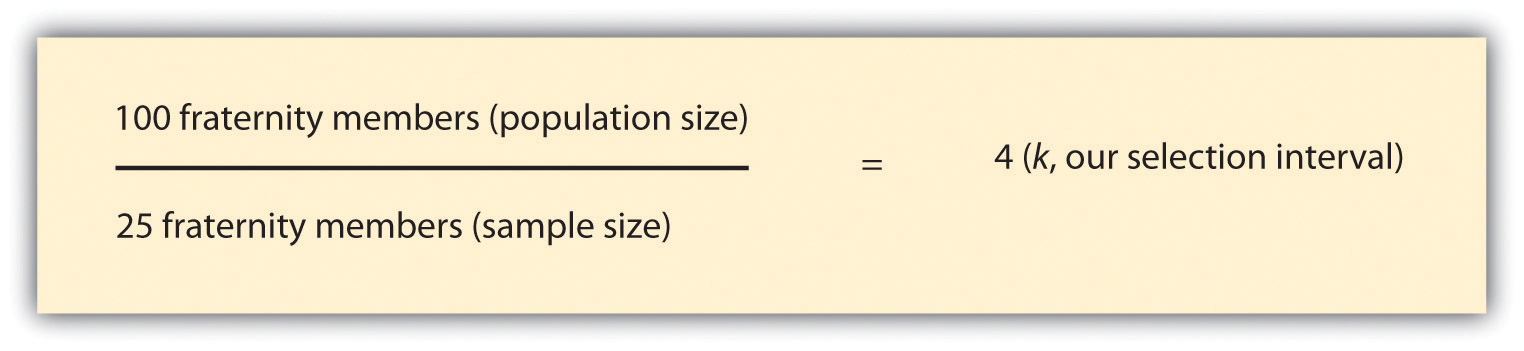
To determine where on your list of accessible population elements to begin selecting the names of the 25 men you will interview, select a random number between 1 and k, and begin there. If we randomly select 3 as our starting point, we’d begin by selecting the third fraternity member on the list and then select every fourth member from there. Table 6.2 lists the names of our hypothetical 100 fraternity members on campus. You’ll see that the third name on the list has been selected for inclusion in our hypothetical study, as has every fourth name after that. A total of 25 names have been selected.

Table 6.2 Systematic Sample of 25 Fraternity Members

Number	Name	Include in study?
1	Jacob
2	Ethan
3	Michael	Yes
4	Jayden
5	William
6	Alexander
7	Noah	Yes
8	Daniel
9	Aiden
10	Anthony
11	Joshua	Yes
12	Mason
13	Christopher
14	Andrew

(Note: Table abbreviated for length, but the pattern of selecting every 4th element continues through 100).

There is one clear instance in which systematic sampling should not be employed. If your sampling frame has any pattern to it, you could inadvertently introduce bias into your sample by using a systemic sampling strategy. This is sometimes referred to as the problem of periodicity. Periodicity refers to the tendency for a pattern to occur at regular intervals. Let’s say, for example, that you wanted to observe how people use the outdoor public spaces on your campus. Perhaps you need to have your observations completed within 28 days and you wish to conduct four observations on randomly chosen days. Table 6.3 shows a list of the population elements for this example. To determine which days we’ll conduct our observations, we’ll need to determine our selection interval. As you’ll recall from the preceding paragraphs, to do so we must divide our population size, in this case 28 days, by our desired sample size, in this case 4 days. This formula leads us to a selection interval of 7. If we randomly select 2 as our starting point and select every seventh day after that, we’ll wind up with a total of 4 days on which to conduct our observations. You’ll see how that works out in the following table.

Table 6.3 Systematic Sample of Observation Days

Number	Day	Include in study?		Number	Day	Include in study?
1	Monday			15	Monday
2	Tuesday	Yes		16	Tuesday	Yes
3	Wednesday			17	Wednesday
4	Thursday			18	Thursday
5	Friday			19	Friday
6	Saturday			20	Saturday
7	Sunday			21	Sunday
8	Monday			22	Monday
9	Tuesday	Yes		23	Tuesday	Yes
10	Wednesday			24	Wednesday
11	Thursday			25	Thursday
12	Friday			26	Friday
13	Saturday			27	Saturday
14	Sunday			28	Sunday

Do you notice any problems with our selection of observation days? Apparently we’ll only be observing on Tuesdays. As you have probably figured out, that isn’t such a good plan if we really wish to understand how public spaces on campus are used. Weekend use probably differs from weekday use, and use may even vary during the week, just as class schedules do. In cases such as this, where the sampling frame is cyclical, it would be better to use a stratified random sampling technique.

3. Stratified Random Sampling

In stratified random sampling, a researcher will divide the study population into relevant subgroups and then draw a sample from each subgroup. Once we have our subgroups, we can then apply either simple random or systematic sampling techniques to each subgroup.

Stratified sampling is a good technique to use when a subgroup of interest makes up a relatively small proportion of the overall sample. For example, in a study analyzing the impacts of modern remote work structures on higher education personnel, researchers might find that administrative adjuncts represent a small but vital stratum compared to full-time faculty. By dividing the institutional database into those distinct strata and randomly selecting from each, the research ensures that unique structural viewpoints are accurately represented in exact proportion to the larger population.

4. Cluster Sampling

Up to this point in our discussion of probability samples, we’ve assumed that researchers will be able to access a list of population elements in order to create a sampling frame. This is not always the case. When attempting to create a list of an entire population is impossible or impractical, researchers turn to cluster sampling. Cluster sampling occurs when a researcher begins by sampling groups (or clusters) of population elements and then selects elements from within those groups. For example, if you want to study organizational trust dynamics among public school educators across a wide geographic region, a complete list of individual teachers may be unavailable. However, a complete list of school districts (the clusters) can easily be obtained. A researcher could randomly sample 15 school districts first, and then randomly sample individual educators within those specific districts. Cluster sampling works in stages; in this example, we sampled in two stages. While sampling in multiple stages does introduce the possibility of greater error, it is nevertheless a highly efficient method.

A clear empirical application of multi-stage cluster sampling can be found in a study by Md. Saidur Rashid Sumon and Md. Shahinuzzaman (2025), who investigated the relationship between social networks, structural community engagement, and altruistic behavior among youth. Because compiling an individualized sampling frame of every young person active in regional community organizations was unfeasible, the researchers utilized a multi-stage cluster approach. They first localized clusters of organized social groups across specified geographical zones, randomly drawing 42 distinct social organizations to serve as their primary sampling units. From within those selected clusters, they systematically sampled 612 individual youth participants to receive their structured questionnaires.

Because civic clusters and local organizations vary vastly in membership size, drawing an identical, flat baseline of participants from every single cluster without adjustment would give youth in smaller organizations a mathematically higher probability of being picked. To ensure every individual member across the broader target population maintained an equal, non-zero chance of selection, researchers utilizing cluster approaches often rely on probability proportionate to size (PPS). This methodology weights a cluster’s likelihood of selection relative to its overall baseline volume, keeping the core principles of random probability sampling intact even across complex, unequal structural groupings.

 

Just to review consider Table 6.4 which details all the sample types.

Table 6.4 Types of Probability Samples

Sample type	Description
Simple random	Researcher randomly selects elements from the sampling frame.
Systematic random	Researcher selects every kth element from the sampling frame.
Stratified random	Researcher creates subgroups and then randomly selects elements from each subgroup.
Cluster	Researcher randomly selects clusters and then randomly selects elements from the selected clusters.

Key Takeaways

• Representation is Key: In probability sampling, the aim is to identify a sample that resembles the population from which it was drawn.

• Variety of Techniques: There are several types of probability samples including simple random samples, systematic samples, stratified samples, and cluster samples.

Exercises

1. Apply the Methods: Imagine that you are about to conduct a study of people’s use of public parks. Explain how you could employ each of the probability sampling techniques described earlier to recruit a sample for your study.

2. Evaluate the Methods: Of the four probability sample types described, which seems strongest to you? Which seems weakest? Explain.