3. Data Cleaning

All original data sets are messy and need to be cleaned to be analyzed effectively. As mentioned in the prerequisites section, the package tidyverse is a great tool to use to clean a data set. There is a plethora of commands and styles of data-cleaning, but we are only going to highlight some basic functions that may be useful for an undergraduate-level research methods course. 

Packages Within the Tidyverse

• ggplot2: grammar of graphics to visualize your data
• dplyr: grammar of data manipulation to solve the most common manipulations
• tidyr: helps to create tidy data
• readr: read rectangular data in an easier way
• purr: provides a complete and consistent toolkit for working with vectors and functions.
• tibble: re-imagines the data frame
• stringr: provides functions that make working with strings as easy as possible
• forcats: provides useful tools to solve problems with factors

For the purposes of this course, you will not need to use all of the packages included in the tidyverse. It is important, however, to be aware of everything that a package can do for you. 

Note

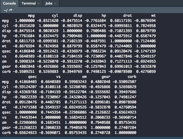
When using tidyverse, the pipe (%>%) is your best friend. This will allow you take one object and perform a sequence of actions on them. The code below is an example of using the built-in dataset mtcars and running a correlation between its variables.

mtcars %>%
    cor()

 

 

dplyr

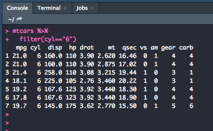
filter(): Select a subset of rows in a dataset. 

Below, we are using the dataset mtcars which is data extracted from a 1974 US magazine that comprises fuel consumption and 10 aspects of automobile design and performance for 32 automobiles. Let's say that we only want to look at the cars that have 6 cylinders on the list.

mtcars %>%
    filter(cyl=="6")

This is what your output should be in the console, only the rows which have a value of "6" in the cyl column. 

You can also add more things to be filtered to make your subset more specific. For example, let's make a subset of cars that have 6 cylinders and have more than 1 carburetor.

mtcars %>%
    filter(cyl=="6",
           carb > 1)       

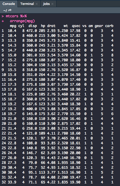
arrange(): Sorts the observations in ascending or descending order based on a variable. 

Let's sort the dataset so that it was in order, low to high, for miles per gallon.

mtcars %>%
    arrange(mpg)

The output in the console should, thus, give you a list of observations arranged by mpg.

You can also arrange observations so that they run high to low using the following code:

mtcars %>%
    arrange(desc(mpg))

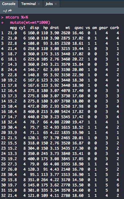
mutate(): Update or create new columns in a data frame

Sometimes when working with a dataset, you need to manipulate variables for analysis. Let's mutate the wt (weight) column so that it reads in lbs, not 1000 lbs. 

mtcars %>%
    mutate(wt=wt*1000 )

 

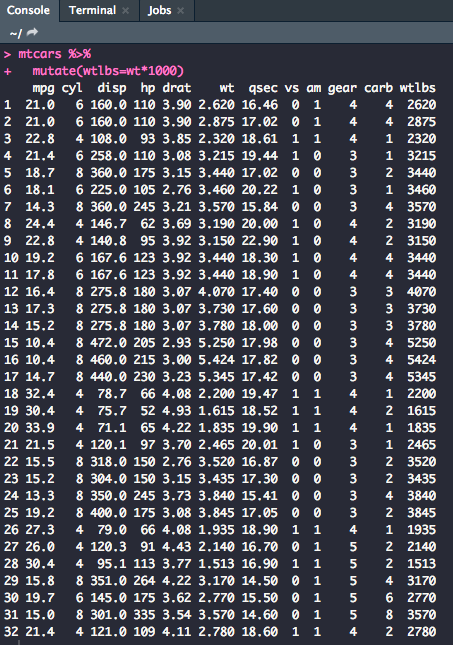
You could also create a new column with the mutated variable.

mtcars %>%
    mutate(wtlbs=wt*1000)

 

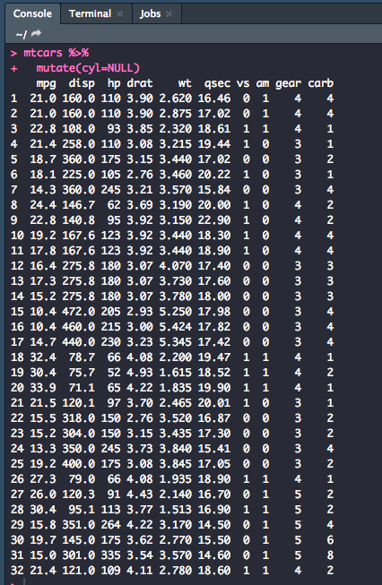
You can also remove variables with the mutate function. Let's get rid of the cyl variable.

mtcars %>%
    mutate(cyl=NULL)

 

Note

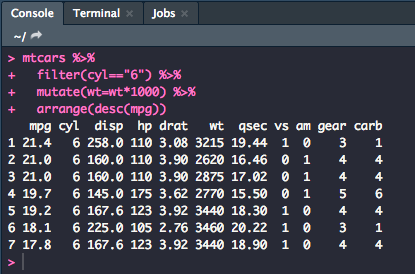
You can also combine verbs using multiple pipes. Let's combine filter(), arrange(), and mutate(). This is part of what makes the tidyverse especially useful.

mtcars %>%
    filter(cyl=="6") %>%
    mutate(wt=wt*1000) %>%
    arrange(desc(mpg))

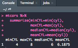
summarize(): Allows you to turn multiple observations into a single data point.

This function is useful for finding values like the minimum, maximum, median, and mean

mtcars %>%
    summarize(minMPG=min(mpg),
              maxMPG=max(mpg),
              medianMPG=median(mpg),
              meanMPG=mean(mpg))

 

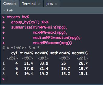
group_by(): Allows you to summarize within groups instead of the entire data set.

mtcars %>%
    group_by(cyl) %>%
    summarize(minMPG=min(mpg),
              maxMPG=max(mpg),
              medianMPG=median(mpg),
              meanMPG=mean(mpg))

 

 

Putting It All Together

Once you have cleaned the data to your desire, you will want to make sure that you save this new version of the dataset as a new .csv file to use in an analysis script. 

After every change that you make to the script, you will want to make an object in the global environment or change an existing one. For example, if we wanted to mutate the wt column to read in lbs then remove the vs column and write a new .csv to reflect the newly cleaned data, we would use the following code: 

mtcars %>%
    mutate(wt = wt*10000) %>%
    mutate(vs = NULL) -> dat

write_csv(dat, "mtcars_clean.csv")

It's important to always choose a descriptive name for your new dataset that isn't the same as the dataset that you pulled it from. Having a copy of the unclean and the clean data will be helpful in case something went wrong in your cleaning efforts. With the new .csv, you can read it into a new script and start analysis!