1.1: Basic Definitions and Concepts
- Page ID
- 19010
Skills to Develop
- To learn the basic definitions used in statistics and some of its key concepts.
We begin with a simple example. There are millions of passenger automobiles in the United States. What is their average value? It is obviously impractical to attempt to solve this problem directly by assessing the value of every single car in the country, add up all those values, then divide by the number of values, one for each car. In practice the best we can do would be to estimate the average value. A natural way to do so would be to randomly select some of the cars, say \(200\) of them, ascertain the value of each of those cars, and find the average of those \(200\) values. The set of all those millions of vehicles is called the population of interest, and the number attached to each one, its value, is a measurement. The average value is a parameter: a number that describes a characteristic of the population, in this case monetary worth. The set of \(200\) cars selected from the population is called a sample, and the \(200\) numbers, the monetary values of the cars we selected, are the sample data. The average of the data is called a statistic: a number calculated from the sample data. This example illustrates the meaning of the following definitions.
Definitions: populations and samples
A population is any specific collection of objects of interest. A sample is any subset or subcollection of the population, including the case that the sample consists of the whole population, in which case it is termed a census.
Definitions: measurements and Sample Data
A measurement is a number or attribute computed for each member of a population or of a sample. The measurements of sample elements are collectively called the sample data.
Definition: parameters
A parameter is a number that summarizes some aspect of the population as a whole. A statistic is a number computed from the sample data.
Continuing with our example, if the average value of the cars in our sample was \($8,357\), then it seems reasonable to conclude that the average value of all cars is about \($8,357\). In reasoning this way we have drawn an inference about the population based on information obtained from the sample. In general, statistics is a study of data: describing properties of the data, which is called descriptive statistics, and drawing conclusions about a population of interest from information extracted from a sample, which is called inferential statistics. Computing the single number \($8,357\) to summarize the data was an operation of descriptive statistics; using it to make a statement about the population was an operation of inferential statistics.
Definition: Statistics
Statistics is a collection of methods for collecting, displaying, analyzing, and drawing conclusions from data.
Definition: Descriptive statistics
Descriptive statistics is the branch of statistics that involves organizing, displaying, and describing data.
Definition: Inferential statistics
Inferential statistics is the branch of statistics that involves drawing conclusions about a population based on information contained in a sample taken from that population.
Definition: Qualitative data
Qualitative data are measurements for which there is no natural numerical scale, but which consist of attributes, labels, or other non-numerical characteristics.
Definition: Quantitative data
Quantitative data are numerical measurements that arise from a natural numerical scale.
Qualitative data can generate numerical sample statistics. In the automobile example, for instance, we might be interested in the proportion of all cars that are less than six years old. In our same sample of \(200\) cars we could note for each car whether it is less than six years old or not, which is a qualitative measurement. If \(172\) cars in the sample are less than six years old, which is \(0.86\) or \(86\% \), then we would estimate the parameter of interest, the population proportion, to be about the same as the sample statistic, the sample proportion, that is, about \(0.86\).
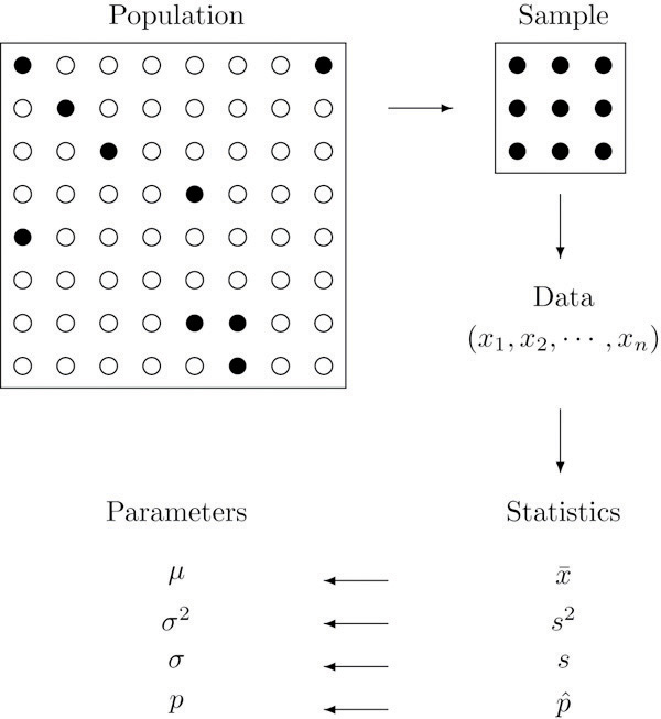
The relationship between a population of interest and a sample drawn from that population is perhaps the most important concept in statistics, since everything else rests on it. This relationship is illustrated graphically in Figure \(\PageIndex{1}\). The circles in the large box represent elements of the population. In the figure there was room for only a small number of them but in actual situations, like our automobile example, they could very well number in the millions. The solid black circles represent the elements of the population that are selected at random and that together form the sample. For each element of the sample there is a measurement of interest, denoted by a lower case \(x\) (which we have indexed as \(x_1 , \ldots, x_n\) to tell them apart); these measurements collectively form the sample data set. From the data we may calculate various statistics. To anticipate the notation that will be used later, we might compute the sample mean \(\bar{x}\) and the sample proportion \(\hat{p}\), and take them as approximations to the population mean \(\mu\) (this is the lower case Greek letter mu, the traditional symbol for this parameter) and the population proportion \(p\), respectively. The other symbols in the figure stand for other parameters and statistics that we will encounter.

Figure \(\PageIndex{1}\): The Grand Picture of Statistics
Key Takeaway
- Statistics is a study of data: describing properties of data (descriptive statistics) and drawing conclusions about a population based on information in a sample (inferential statistics).
- The distinction between a population together with its parameters and a sample together with its statistics is a fundamental concept in inferential statistics.
- Information in a sample is used to make inferences about the population from which the sample was drawn.

