When examining economic statistics, there is a crucial distinction worth emphasizing. The distinction is between nominal and real measurements, which refer to whether or not inflation has distorted a given statistic. Looking at economic statistics without considering inflation is like looking through a pair of binoculars and trying to guess how close something is: unless you know how strong the lenses are, you cannot guess the distance very accurately. Similarly, if you do not know the rate of inflation, it is difficult to figure out if a rise in GDP is due mainly to a rise in the overall level of prices or to a rise in quantities of goods produced. The nominal valueof any economic statistic means the statistic is measured in terms of actual prices that exist at the time. The real value refers to the same statistic after it has been adjusted for inflation. Generally, it is the real value that is more important.
Converting Nominal to Real GDP
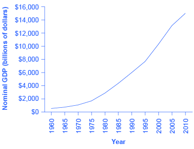
Table 1 shows U.S. GDP at five-year intervals since 1960 in nominal dollars; that is, GDP measured using the actual market prices prevailing in each stated year. This data is also reflected in the graph shown in Figure 1
Year
Nominal GDP (billions of dollars)
GDP Deflator (2005 = 100)
1960
543.3
19.0
1965
743.7
20.3
1970
1,075.9
24.8
1975
1,688.9
34.1
1980
2,862.5
48.3
1985
4,346.7
62.3
1990
5,979.6
72.7
1995
7,664.0
81.7
2000
10,289.7
89.0
2005
13,095.4
100.0
2010
14,958.3
110.0
Table 1: U.S. Nominal GDP and the GDP Deflator(Source: www.bea.gov)
U.S. Nominal GDP, 1960–2010
Figure 1: Nominal GDP values have risen exponentially from 1960 through 2010, according to the BEA.
If an unwary analyst compared nominal GDP in 1960 to nominal GDP in 2010, it might appear that national output had risen by a factor of twenty-seven over this time (that is, GDP of $14,958 billion in 2010 divided by GDP of $543 billion in 1960). This conclusion would be highly misleading. Recall that nominal GDP is defined as the quantity of every good or service produced multiplied by the price at which it was sold, summed up for all goods and services. In order to see how much production has actually increased, we need to extract the effects of higher prices on nominal GDP. This can be easily done, using the GDP deflator.
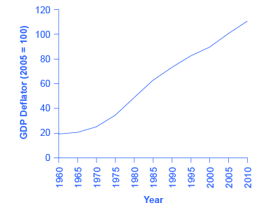
GDP deflatoris a price index measuring the average prices of all goods and services included in the economy. We explore price indices in detail and how they are computed in Inflation, but this definition will do in the context of this chapter. The data for the GDP deflator are given in Table 1 and shown graphically in Figure 2.
U.S. GDP Deflator, 1960–2010
Figure 2: Much like nominal GDP, the GDP deflator has risen exponentially from 1960 through 2010. (Source: BEA)
Figure 2 shows that the price level has risen dramatically since 1960. The price level in 2010 was almost six times higher than in 1960 (the deflator for 2010 was 110 versus a level of 19 in 1960). Clearly, much of the apparent growth in nominal GDP was due to inflation, not an actual change in the quantity of goods and services produced, in other words, not in real GDP. Recall that nominal GDP can rise for two reasons: an increase in output, and/or an increase in prices. What is needed is to extract the increase in prices from nominal GDP so as to measure only changes in output. After all, the dollars used to measure nominal GDP in 1960 are worth more than the inflated dollars of 1990—and the price index tells exactly how much more. This adjustment is easy to do if you understand that nominal measurements are in value terms, where
\[Value=Price\,\times\,Quantity\]
\[or\]
\[Nominal\,GDP=GDP\,Deflator\,\times\,Real\,GDP\]
Let’s look at an example at the micro level. Suppose the t-shirt company, Coolshirts, sells 10 t-shirts at a price of $9 each.
In other words, when we compute “real” measurements we are trying to get at actual quantities, in this case, 10 t-shirts.
With GDP, it is just a tiny bit more complicated. We start with the same formula as above:
\[Real\,GDP=\dfrac{Nominal\,GDP}{Price\,Index}\]
For reasons that will be explained in more detail below, mathematically, a price index is a two-digit decimal number like 1.00 or 0.85 or 1.25. Because some people have trouble working with decimals, when the price index is published, it has traditionally been multiplied by 100 to get integer numbers like 100, 85, or 125. What this means is that when we “deflate” nominal figures to get real figures (by dividing the nominal by the price index). We also need to remember to divide the published price index by 100 to make the math work. So the formula becomes:
We’ll do this in two parts to make it clear. First adjust the price index: 19 divided by 100 = 0.19. Then divide into nominal GDP: $543.3 billion / 0.19 = $2,859.5 billion.
Step 3. Use the same formula to calculate the real GDP in 1965.
Step 4. Continue using this formula to calculate all of the real GDP values from 1960 through 2010. The calculations and the results are shown in Table 2.
Year
Nominal GDP (billions of dollars)
GDP Deflator (2005 = 100)
Calculations
Real GDP (billions of 2005 dollars)
1960
543.3
19.0
543.3 / (19.0/100)
2859.5
1965
743.7
20.3
743.7 / (20.3/100)
3663.5
1970
1075.9
24.8
1,075.9 / (24.8/100)
4338.3
1975
1688.9
34.1
1,688.9 / (34.1/100)
4952.8
1980
2862.5
48.3
2,862.5 / (48.3/100)
5926.5
1985
4346.7
62.3
4,346.7 / (62.3/100)
6977.0
1990
5979.6
72.7
5,979.6 / (72.7/100)
8225.0
1995
7664.0
82.0
7,664 / (82.0/100)
9346.3
2000
10289.7
89.0
10,289.7 / (89.0/100)
11561.5
2005
13095.4
100.0
13,095.4 / (100.0/100)
13095.4
2010
14958.3
110.0
14,958.3 / (110.0/100)
13598.5
Table 2: Converting Nominal to Real GDP(Source: Bureau of Economic Analysis, www.bea.gov)
There are a couple things to notice here. Whenever you compute a real statistic, one year (or period) plays a special role. It is called the base year (or base period). The base year is the year whose prices are used to compute the real statistic. When we calculate real GDP, for example, we take the quantities of goods and services produced in each year (for example, 1960 or 1973) and multiply them by their prices in the base year (in this case, 2005), so we get a measure of GDP that uses prices that do not change from year to year. That is why real GDP is labeled “Constant Dollars” or “2005 Dollars,” which means that real GDP is constructed using prices that existed in 2005. The formula used is:
Comparing real GDP and nominal GDP for 2005, you see they are the same. This is no accident. It is because 2005 has been chosen as the “base year” in this example. Since the price index in the base year always has a value of 100 (by definition), nominal and real GDP are always the same in the base year.
Use this data to make another observation: As long as inflation is positive, meaning prices increase on average from year to year, real GDP should be less than nominal GDP in any year after the base year. The reason for this should be clear: The value of nominal GDP is “inflated” by inflation. Similarly, as long as inflation is positive, real GDP should be greater than nominal GDP in any year before the base year.
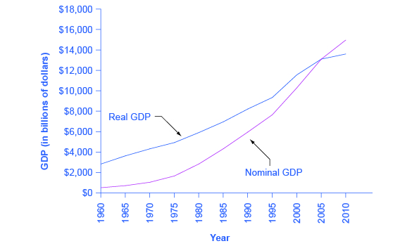
Figure 3 shows the U.S. nominal and real GDP since 1960. Because 2005 is the base year, the nominal and real values are exactly the same in that year. However, over time, the rise in nominal GDP looks much larger than the rise in real GDP (that is, the nominal GDP line rises more steeply than the real GDP line), because the rise in nominal GDP is exaggerated by the presence of inflation, especially in the 1970s.
U.S. Nominal and Real GDP, 1960–2012
Figure 3: The red line measures U.S. GDP in nominal dollars. The black line measures U.S. GDP in real dollars, where all dollar values have been converted to 2005 dollars. Since real GDP is expressed in 2005 dollars, the two lines cross in 2005. However, real GDP will appear higher than nominal GDP in the years before 2005, because dollars were worth less in 2005 than in previous years. Conversely, real GDP will appear lower in the years after 2005, because dollars were worth more in 2005 than in later years.
Let’s return to the question posed originally: How much did GDP increase in real terms? What was the rate of growth of real GDP from 1960 to 2010? To find the real growth rate, we apply the formula for percentage change:
In other words, the U.S. economy has increased real production of goods and services by nearly a factor of four since 1960. Of course, that understates the material improvement since it fails to capture improvements in the quality of products and the invention of new products.
There is a quicker way to answer this question approximately, using another math trick. Because:
Therefore, the growth rate of real GDP (% change in quantity) equals the growth rate in nominal GDP (% change in value) minus the inflation rate (% change in price).
Note that using this equation provides an approximation for small changes in the levels. For more accurate measures, one should use the first formula shown.
Key Concepts and Summary
The nominal value of an economic statistic is the commonly announced value. The real value is the value after adjusting for changes in inflation. To convert nominal economic data from several different years into real, inflation-adjusted data, the starting point is to choose a base year arbitrarily and then use a price index to convert the measurements so that they are measured in the money prevailing in the base year.
Glossary
nominal value
the economic statistic actually announced at that time, not adjusted for inflation; contrast with real value
real value
an economic statistic after it has been adjusted for inflation; contrast with nominal value