3.2: The Market's Building Blocks

In economics we use the terminology that describes trade in a particular manner. Non-economists frequently describe microeconomics by saying “it’s all about supply and demand”. While this is largely true we need to define exactly what we mean by these two central words. Let’s start with demand. Demand is the quantity of a good or service that buyers wish to purchase at each conceivable price, with all other influences on demand remaining unchanged. It reflects a multitude of values, not a single value. It is not a single or unique quantity such as two cell phones, but rather a full description of the quantity of a good or service that buyers would purchase at various prices.

Demand is the quantity of a good or service that buyers wish to purchase at each possible price, with all other influences on demand remaining unchanged.

As an example, the first column of Table 3.1 shows the price of natural gas per cubic foot. The second column shows the quantity that would be purchased in a given time period at each price. It is therefore a schedule of prices.

Supply is interpreted in a similar manner. It is not a single value; it is a schedule of the quantity that sellers would want to sell at each price. Hence we say that supply is the quantity of a good or service that sellers are willing to sell at each possible price, with all other influences on supply remaining unchanged. Such a supply schedule is defined in the third column of the table. It is assumed that no supplier can make a profit (on account of their costs) unless the price is at least $2 per unit, and therefore a zero quantity is supplied below that price. The higher price is more profitable, and therefore induces a greater quantity supplied, perhaps by attracting more suppliers.

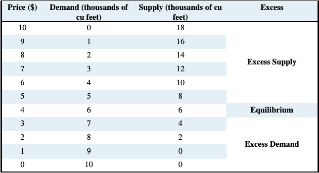
Table 3.1: Demand and Supply for Natural Gas

Supply is the quantity of a good or service that sellers are willing to sell at each possible price, with all other influences on supply remaining unchanged.

We can now identify a key difference in terminology – between the words demand and quantity demanded, and between supply and quantity supplied. While the words demand and supply refer to the complete schedules of demand and supply, the terms quantity demanded and quantity supplied each define a single value of demand or supply at a particular price.

Quantity demanded defines the amount purchased at a particular price.

Quantity supplied refers to the amount supplied at a particular price.

Thus while the non-economist may say that when some fans did not get tickets to the Stanley Cup it was a case of demand exceeding supply, as economists we say that the quantity demanded exceeded the quantity supplied at the going price of tickets. In this instance, had every ticket been offered at a sufficiently high price, the market could have generated an excess supply rather than an excess demand. A higher ticket price would reduce the quantity demanded; yet would not change demand, because demand refers to the whole schedule of possible quantities demanded at different prices.

Other things equal – ceteris paribus

The demand and supply schedules rest on the assumption that all other influences on supply and demand remain the same as we move up and down the possible price values. We use the expression other things being equal, or its Latin counterpart ceteris paribus, to describe this constancy of other influences. For example, we assume on the demand side that the prices of other goods remain constant, that tastes and incomes are unchanging, that the size of the market is given, and so forth. On the supply side we assume, for example, that there is no technological change in production methods.

Market equilibrium

Let us now bring the demand and supply schedules together in an attempt to analyze what the market place will produce – will a single price emerge that will equate supply and demand? We will keep other things constant for the moment, and explore what materializes at different prices. At low prices, the data in Table 3.1 indicate that the quantity demanded exceeds the quantity supplied – for example, verify what happens when the price is $3 per unit. The opposite occurs when the price is high – what would happen if the price were $8? Evidently, there exists an intermediate price, where the quantity demanded equals the quantity supplied. At this point we say that the market is in equilibrium. The equilibrium price equates demand and supply – it clears the market.

The equilibrium price equilibrates the market. It is the price at which quantity demanded equals the quantity supplied.

In Table 3.1 the equilibrium price is $4, and the equilibrium quantity is 6 thousand cubic feet of gas (we will use the notation ‘k’ to denote thousands). At higher prices there is an excess supply— suppliers wish to sell more than buyers wish to buy. Conversely, at lower prices there is an excess demand. Only at the equilibrium price is the quantity supplied equal to the quantity [demanded].

Excess supply exists when the quantity supplied exceeds the quantity demanded at the going price.

Excess demand exists when the quantity demanded exceeds the quantity supplied at the going price.

Does the market automatically reach equilibrium? To answer this question, suppose initially that the sellers choose a price of $10. Here suppliers would like to supply 18k cubic feet, but there are no buyers—a situation of extreme excess supply. At the price of $7 the excess supply is reduced to 9k, because both the quantity demanded is now higher at 3k units, and the quantity supplied is lower at 12k. But excess supply means that there are suppliers willing to supply at a lower price, and this willingness exerts continual downward pressure on any price above the price that equates demand and supply.

At prices below the equilibrium there is, conversely, an excess demand. In this situation, suppliers could force the price upward, knowing that buyers will continue to buy at a price at which the suppliers are willing to sell. Such upward pressure would continue until the excess demand is eliminated.

In general then, above the equilibrium price excess supply exerts downward pressure on price, and below the equilibrium excess demand exerts upward pressure on price. This process implies that the buyers and sellers have information on the various elements that make up the marketplace.

Note that, if sales do take place at prices above or below the equilibrium price, the quantity traded always corresponds to the short side of the market: At high prices the quantity demanded is less than supply, and it is the quantity demanded that is traded because buyers will not buy the amount suppliers would like to supply. At low prices the quantity demanded exceeds quantity supplied, and it is the amount that suppliers are willing to sell that is traded. In sum, when trading takes place at prices other than the equilibrium price it is always the lesser of the quantity demanded or supplied that is traded. Hence we say that at non equilibrium prices the short side dominates. We will return to this in a series of examples later in this chapter.

The short side of the market determines outcomes at prices other than the equilibrium.

Supply and the nature of costs

Before progressing to a graphical analysis, we should add a word about costs. The supply schedules are based primarily on the cost of producing the product in question, and we frequently assume that all of the costs associated with supply are incorporated in the supply schedules. In Microeconomics Chapter 6 we will explore cases where costs additional to those incurred by producers may be relevant. For example, coal burning power plants emit pollutants into the atmosphere; but the individual supplier may not take account of these pollutants, which are costs to society at large, in deciding how much to supply at different prices. Stated another way, the private costs of production would not reflect the total, or full social costs of production. For the moment the assumption is that no such additional costs are associated with the markets we analyze.