3.5: Other Influences on Supply

To date we have drawn supply curves with an upward slope. Is this a reasonable representation of supply in view of what is frequently observed in markets? We suggested earlier that the various producers of a particular good or service may have different levels of efficiency. If so, only the more efficient producers can make a profit at a low price, whereas at higher prices more producers or suppliers enter the market – producers who may not be as lean and efficient as those who can survive in a lower-price environment. This view of the world yields an upward-sloping supply curve, although there are other perspectives on the supply curve’s slope.

Frequently producers simply choose a price and let buyers purchase as much as they want at that price. This is the practice of most retailers. For example, the price of Samsung’s Galaxy is typically fixed, no matter how many are purchased – and tens of millions are sometimes sold at a fixed price when a new model is launched. Apple sets a price, and buyers purchase as many as they desire at that price.

In yet other situations supply is fixed. This happens in auctions, and bidders at the auction simply determine the price to be paid. At a real estate auction a fixed number of homes are put on the market and prices are determined by the bidding process.

Regardless of the type of market we encounter, however, it is safe to assume that supply curves do not slope downward. So, for the moment, we adopt the stance that supply curves are generally upward sloping – somewhere between the extremes of being vertical or horizontal – as we have drawn them to this point.

Next, we examine those other influences that underlie supply curves. Technology, input costs, the prices of competing goods, expectations and the number of suppliers are the most important.

Technology

A technological advance may involve an idea that allows more output to be produced with the same inputs, or an equal output with fewer inputs. A good example is just-in-time technology. Before the modern era, auto manufacturers kept large stocks of components in their production facilities, but developments in communications and computers at that time made it possible for manufacturers to link directly with their input suppliers. Nowadays assembly plants place their order for, say, seat delivery to their local seat supplier well ahead of time. The seats swing into the assembly area hours or minutes before assembly—just in time. The result is that the assembler reduces his seat inventory (an input) and thereby reduces production cost.

Such a technology-induced cost saving is represented by moving the supply curve downward or outward: The supplier is willing to supply the same quantity at a lower price because of the technological innovation. Or, saying the same thing slightly differently, suppliers will supply more at a given price than before. This is but one example of how “supply chains” are evolving in the modern globalized world. Computer assemblers are prime examples of the same developments.

Input costs

Input costs can vary independently of technology. For example, a wage negotiation that grants workers an increase above the general inflation rate will increase the cost of production. This is reflected in a leftward, or upward, supply shift: Any quantity is now priced higher; alternatively, suppliers are willing to supply less at the going price.

As a further example, suppose the government decrees that power-generating companies must provide a certain percentage of their power using ‘green’ sources – from solar power or windmills. Since such sources are not yet as cost efficient as more conventional power sources, the electricity they generate comes at a higher cost.

Competing products

If competing products improve in quality or fall in price, a supplier may be forced to follow suit. For example, Hewlett-Packard and Dell are constantly watching each other’s pricing policies. If Dell brings out a new generation of computers at a lower price, Hewlett-Packard will likely lower its prices in turn—which is to say that Hewlett-Packard’s supply curve will shift downward. Likewise, Samsung and Apple each responds to the other’s pricing and technology behaviours.

These are some of the many factors that influence the position of the supply curve in a given market.

Technological developments have had a staggering impact on many price declines. Professor William Nordhaus of Yale University is an expert on measuring technological change. He has examined the trend in the real price of lighting. Originally, light was provided by whale oil and gas lamps and these sources of lumens (the scientific measure of the amount of light produced) were costly. In his research, Professor Nordhaus pieced together evidence on the actual historic cost of light produced at various times, going all the way back to 1800. He found that light in 1800 cost about 100 times more than in 1900, and light in the year 2000 was a fraction of its cost in 1900. A rough calculation suggests that light was five hundred times more expensive at the start of this 200-year period than at the end.

In terms of supply and demand analysis, light has been subject to very substantial downward supply shifts. Despite the long-term growth in demand, the technologically-induced supply changes have been the dominant factor in its price determination.

For further information, visit Professor Nordhaus’s website in the Department of Economics at Yale University.

Shifts in supply

Whenever technology changes, or the costs of production change, or the prices of competing products adjust, then one of our ceteris paribus assumptions is violated. Such changes are generally reflected by shifting the supply curve. Figure 3.3 illustrates the impact of the arrival of just-in-time technology. The supply curve shifts, reflecting the ability of suppliers to supply the same output at a reduced price. The resulting new equilibrium price is lower, since production costs have fallen. At this reduced price more gas is traded at a lower price.

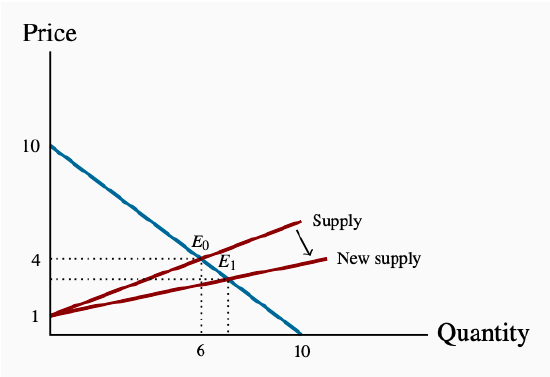
Figure 3.3: Supply Shift and New Equilibrium
The supply curve shifts due to lower production costs. A new equilibrium
E₁ is attained in the market at a lower price.