3.6: Simultaneous Supply and Demand Impacts

Last updated
Save as PDF

Page ID: 11800

$ \newcommand{\vecs}[1]{\overset { \scriptstyle \rightharpoonup} {\mathbf{#1}} } $ $ \newcommand{\vecd}[1]{\overset{-\!-\!\rightharpoonup}{\vphantom{a}\smash {#1}}} $$\newcommand{\id}{\mathrm{id}}$ $ \newcommand{\Span}{\mathrm{span}}$ $ \newcommand{\kernel}{\mathrm{null}\,}$ $ \newcommand{\range}{\mathrm{range}\,}$ $ \newcommand{\RealPart}{\mathrm{Re}}$ $ \newcommand{\ImaginaryPart}{\mathrm{Im}}$ $ \newcommand{\Argument}{\mathrm{Arg}}$ $ \newcommand{\norm}[1]{\| #1 \|}$ $ \newcommand{\inner}[2]{\langle #1, #2 \rangle}$ $ \newcommand{\Span}{\mathrm{span}}$ $\newcommand{\id}{\mathrm{id}}$ $ \newcommand{\Span}{\mathrm{span}}$ $ \newcommand{\kernel}{\mathrm{null}\,}$ $ \newcommand{\range}{\mathrm{range}\,}$ $ \newcommand{\RealPart}{\mathrm{Re}}$ $ \newcommand{\ImaginaryPart}{\mathrm{Im}}$ $ \newcommand{\Argument}{\mathrm{Arg}}$ $ \newcommand{\norm}[1]{\| #1 \|}$ $ \newcommand{\inner}[2]{\langle #1, #2 \rangle}$ $ \newcommand{\Span}{\mathrm{span}}$$\newcommand{\AA}{\unicode[.8,0]{x212B}}$

In the real world, demand and supply frequently shift at the same time. We present two very real such cases in Figures 3.4 and 3.5.

Figure 3.4 is a development of the gas market already discussed. In 2003/04 the price of oil sat at about $30 US per barrel. By the end of the decade it had climbed to $100 per barrel. During the same period the price of natural gas dropped from the $8 per unit range to $3 per unit. A major factor in generating this decline was the development of new ‘fracking’ technologies – the retrieval of gas from shale formations. These technologies are not widespread in Canada due to concerns about their environmental impact, but have been adopted on a large scale in the US. Cheaper production has led to a substantial shift in supply, at the same time as users were demanding more gas due to the rising price of oil. Figure 3.4 illustrates a simultaneous shift in both functions, with the dominant impact coming from the supply side.

Our second example comes from data on a small Montreal municipality. Vertical curves define the supply side of the market. Such vertical curves mean that a fixed number of homeowners decide to put their homes on the market, and these suppliers just take whatever price results in the market. In this example, fewer houses were offered for sale in 2002 (less than 50) than in 1997 (more than 70).

During this time period household incomes increased substantially and, also, mortgage rates fell. Both of these developments shifted the demand curve upward/outward: buyers were willing to pay more for housing in 2002 than in 1997. The higher price in 2002 was therefore due to both demand and supply side shifts in the marketplace.

Screenshot 2019-02-21 at 23.37.50.png

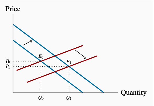
Figure 3.4: Simultaneous Demand and Supply Shifts
The outward shift in supply dominates the outward shift in demand, leading
to a new equilibrium E1 at a lower price and higher quantity.

Screenshot 2019-02-21 at 23.40.20.png

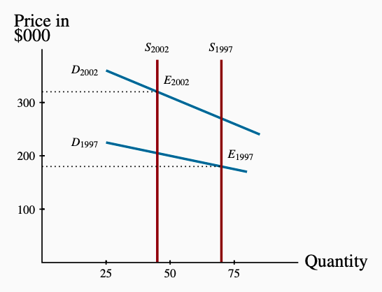
Figure 3.5: A Model of the Housing Market with Shifts in Demand and Supply
The vertical supply denotes a fixed number of houses supplied each year.
Demand was stronger in 2002 than in 1997 both on account of higher in-
comes and lower mortgage rates. Thus the higher price in 2002 is due to
both a reduction in supply and an increase in demand.