Exercises for Chapter 3

Last updated
Save as PDF

Page ID: 12741

$ \newcommand{\vecs}[1]{\overset { \scriptstyle \rightharpoonup} {\mathbf{#1}} } $ $ \newcommand{\vecd}[1]{\overset{-\!-\!\rightharpoonup}{\vphantom{a}\smash {#1}}} $$\newcommand{\id}{\mathrm{id}}$ $ \newcommand{\Span}{\mathrm{span}}$ $ \newcommand{\kernel}{\mathrm{null}\,}$ $ \newcommand{\range}{\mathrm{range}\,}$ $ \newcommand{\RealPart}{\mathrm{Re}}$ $ \newcommand{\ImaginaryPart}{\mathrm{Im}}$ $ \newcommand{\Argument}{\mathrm{Arg}}$ $ \newcommand{\norm}[1]{\| #1 \|}$ $ \newcommand{\inner}[2]{\langle #1, #2 \rangle}$ $ \newcommand{\Span}{\mathrm{span}}$ $\newcommand{\id}{\mathrm{id}}$ $ \newcommand{\Span}{\mathrm{span}}$ $ \newcommand{\kernel}{\mathrm{null}\,}$ $ \newcommand{\range}{\mathrm{range}\,}$ $ \newcommand{\RealPart}{\mathrm{Re}}$ $ \newcommand{\ImaginaryPart}{\mathrm{Im}}$ $ \newcommand{\Argument}{\mathrm{Arg}}$ $ \newcommand{\norm}[1]{\| #1 \|}$ $ \newcommand{\inner}[2]{\langle #1, #2 \rangle}$ $ \newcommand{\Span}{\mathrm{span}}$$\newcommand{\AA}{\unicode[.8,0]{x212B}}$

Exercise 3.1 Supply and demand data for concerts are shown below.

Screenshot 2019-02-22 at 13.53.14.png

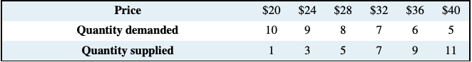
(a) Plot the supply and demand curves to scale and establish the equilibrium price and quantity.

(b) What is the excess supply or demand when price is $24? When price is $36?

(d) The functions underlying the example in the table are linear and can be presented as P = 18 + 2Q (supply) and P = 60 − 4Q (demand). Solve the two equations for the equilibrium price and quantity values.

Exercise 3.2 Illustrate in a supply/demand diagram, by shifting the demand curve appropriately, the effect on the demand for flights between Calgary and Winnipeg as a result of:

(a) Increasing the annual government subsidy to Via Rail.

(b) Improving the Trans-Canada highway between the two cities.

Exercise 3.3 A new trend in U.S. high schools is the widespread use of chewing tobacco. A recent survey indicates that 15 percent of males in upper grades now use it – a figure not far below the use rate for cigarettes. Apparently this development came about in response to the widespread implementation by schools of regulations that forbade cigarette smoking on and around school property. Draw a supply-demand equilibrium for each of the cigarette and chewing tobacco markets before and after the introduction of the regulations.

Exercise 3.4 In Exercise 3.1, suppose there is a simultaneous shift in supply and demand caused by an improvement in technology and a growth in incomes. The technological improvement is represented by a lower supply curve: P = 10 + 2Q. The higher incomes boost demand to P = 76−4Q.

(a) Draw the new supply and demand curves on a diagram and compare them with the pre-change curves.

(b) Equate the new supply and demand functions and solve for the new equilibrium price and quantity.

Exercise 3.5 The market for labour can be described by two linear equations. Demand is given by P = 170−(1/6)Q, and supply is given by P = 50+ (1/3)Q, where Q is the quantity of labour and P is the price of labour – the wage rate.

(a) Graph the functions and find the equilibrium price and quantity by equating demand and supply.

(b) Suppose a price ceiling is established by the government at a price of $120. This price is below the equilibrium price that you have obtained in part a. Calculate the amount that would be demanded and supplied and then calculate the excess demand.

Exercise 3.6 In Exercise 3.5, suppose that the supply and demand describe an agricultural market rather than a labour market, and the government implements a price floor of $140. This is greater than the equilibrium price.

(a) Estimate the quantity supplied and the quantity demanded at this price, and calculate the excess supply.

(b) Suppose the government instead chose to maintain a price of $140 by implementing a system of quotas. What quantity of quotas should the government make available to the suppliers?

Exercise 3.7 In Exercise 3.6, suppose that, at the minimum price, the government buys up all of the supply that is not demanded, and exports it at a price of $80 per unit. Compute the cost to the government of this operation.

Exercise 3.8 Let us sum two demand curves to obtain a ‘market’ demand curve. We will suppose there are just two buyers in the market. The two demands are defined by: P = 42 − (1/3)Q and P = 42−(1/2)Q.

(a) Draw the demands (approximately to scale) and label the intercepts on both the price and quantity axes.

(b) Determine how much would be purchased at prices $10, $20, and $30.

Exercise 3.9 In Exercise 3.8 the demand curves had the same price intercept. Suppose instead that the first demand curve is given by P = 36 − (1/3)Q and the second is unchanged. Graph these curves and illustrate the market demand curve.

Exercise 3.10 Here is an example of a demand curve that is not linear: $P = 5 − 0.2 \sqrt{Q}$. The final term here is the square root of Q.

(a) Draw this function on a graph and label the intercepts. You will see that the price intercept is easily obtained. Can you obtain the quantity intercept where P = 0?

(b) To verify that the shape of your function is correct you can plot this demand curve in a spreadsheet.

Exercise 3.11 The football stadium of the University of the North West Territories has 30 seats. The demand for tickets is given by P = 36−(1/2)Q, where Q is the number of ticket-buying fans.

(a) At the equilibrium admission price how much revenue comes in from ticket sales for each game?

(b) A local fan is offering to install 6 more seats at no cost to the University. Compute the price that would be charged with this new supply and compute the revenue that would accrue each game. Should the University accept the offer to install the seats?

(c) Redo part (b) of this question, assuming that the initial number of seats is 40, and the University has the option to increase capacity to 46 at no cost to itself. Should the University accept the offer in this case?

Exercise 3.12 Suppose farm workers in Mexico are successful in obtaining a substantial wage increase. Illustrate the effect of this on the price of lettuce in the Canadian winter.