6.2: Consumption, Saving, and Investment

Chapter 4 introduced the circular flow of income payments between households and business. Business pays incomes to households to buy factor inputs. Households use income to buy the output of business, providing business revenue. Business revenue is ultimately returned to households as factor incomes. We now build a simple model of this interaction between households and business.

Aggregate expenditure is the sum of planned consumption expenditure by households, investment expenditure by business, and expenditure by residents of other countries on exports of domestic output, minus the imports contained in all these planned expenditures on goods and services. Using AE to denote aggregate expenditure, C for consumption expenditure, I for investment expenditure, X for exports, and IM for imports,

\[ \text{AE} = C + I + X - IM\]

Aggregate expenditure (AE): the sum of planned expenditure in the economy.

Consumption expenditures, investment expenditures, and expenditures on exports of domestic output and imported goods and services are made by different groups and depend on different things. To establish the underlying sources of aggregate expenditure we examine each of its components in more detail.

Consumption Expenditure

Households buy goods and services such as food, cars, movie tickets, internet services and downloads of music and video. Annual consumption expenditures averaged about 90 percent of disposable income and were about 60 percent of GDP in 2013. Disposable income is the income households receive from employment, plus transfer payments received from governments, minus direct taxes they pay to governments. Households decide to either spend or save their disposable incomes.

Disposable income is income net of taxes and transfers.

The scatter diagram of annual data in Figure 6.2 illustrates the relationship between real disposable income and real consumption expenditure in Canada. We know from Chapter 4 that consumption expenditure is the largest component of real GDP measured by the expenditure approach. The slope of the line drawn in the diagram, which passes close to the data points, shows us that a $1 increase in real disposable income results in an increase in real consumption expenditure of about $0.90.

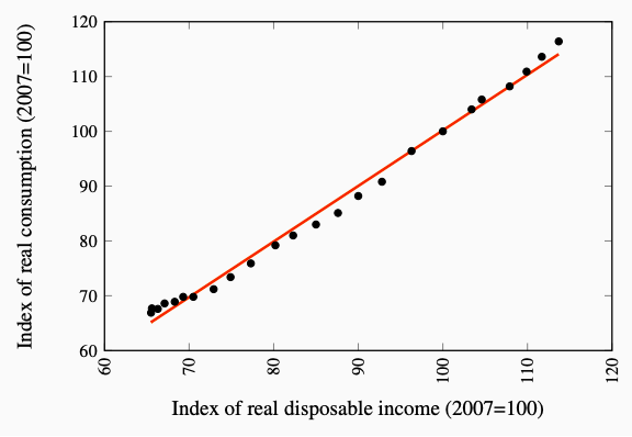
Figure 6.2: A Consumption Function for Canada, 1990-2013 Source: Statistics Canada, CANSIM Tables 380;0064 and 380-0065

Because we have assumed there is no government, disposable income is simply the income households receive from employment in business firms. Each household decides how to allocate its disposable income between spending and saving. Some families save part of their disposable income and accumulate wealth; others spend more and borrow, incurring debt. While consumption and saving decisions depend on many factors, we start with a simple, basic argument. Aggregate consumption expenditure is determined by aggregate disposable income. It rises or falls when disposable income rises or falls, but it does not rise or fall by as much as disposable income rises or falls.

Figure 6.2 shows this positive relationship in the annual data for real consumption expenditure and real disposable income in Canada. Because the scatter of points lies close to an upward sloping line summarizing this relationship, our basic argument is reasonable. Nevertheless, the points do not lie exactly along the line. The simplification we start with omits some other influences on consumption expenditure that we take up later.

The relationship between disposable income and consumption expenditure we see in Figure 6.2 is called the consumption function.

Consumption function: planned consumption expenditure at each level of disposable income.

The consumption function tells us how disposable income Y and consumption expenditure C are related. If C0 is a positive constant, and c is a positive fraction between zero and one,

\[C = C_0 + cY\]

We have assumed for simplicity there is no government that might impose taxes or make transfer payments. As a result disposable income equals national income. Equation 6.2 then relates planned consumption expenditure to national income Y. With c a constant fraction, the consumption function is a straight line.

The intercept C₀ is autonomous consumption expenditure. Autonomous expenditure is not related to current income. Households wish to consume C₀ based on things other than income.

Autonomous expenditure: expenditure not related to current income.

The slope of the consumption function is the marginal propensity to consume. The marginal propensity to consume is the change in consumption expenditure caused by a change in income¹. We call this induced expenditure, and write,

\(\displaystyle\frac {\Delta C}{\Delta Y} = MPC\)

Marginal propensity to consume (MPC): the change in consumption expenditure caused by a change in income.

Induced expenditure: expenditure determined by national income that changes if national income changes.

Table 6.1 and Figure 6.3 illustrate these relationships. Autonomous consumption expenditure, C₀ = 20 in the numerical example, determines the vertical intercept of the function in the diagram. The marginal propensity to consume, c = 0.8, is the slope of the function. You can see in the table that an increase in income by 50 induces an increase in consumption expenditure by 40, which is \(0.8 \times 50\). A change in autonomous consumption expenditure would shift the entire function, changing consumption at every level of income.

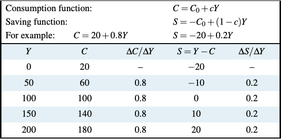
Table 6.1: The Consumption and Saving Functions: A Numerical Example

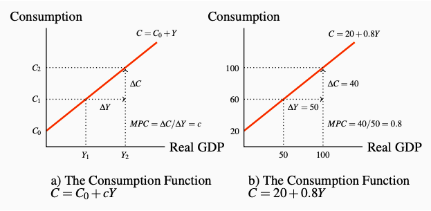
Figure 6.3: The Consumption Function

Saving

Saving is income not spent to finance consumption. Figure 6.3 in Panel a) and Equation 6.2 imply that when income Y is zero, saving is –C₀. Households are not saving, borrowing, or selling their assets.

Because just a fraction c of any change in income is spent on consumption, the remaining fraction \(1 - c\) of any change in income is saved. The marginal propensity to save \(MPS = \displaystyle\frac {\Delta S}{\Delta Y}\) is \(1 - c\). Accordingly a change in income changes planned consumption and planned saving, and \(MPC + MPS = 1\). Figure 6.4 shows the saving function corresponding to the consumption function in Figure 6.3.

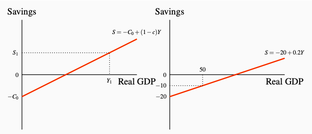
Figure 6.4: The Saving Equation

Marginal propensity to save (MPS): the change in saving caused by a change in income.

Saving function: planned saving at each level of income.

Based on Equation 6.2 and the absence of government and foreign sectors, households can either spend income on consumption or save it. This means \(Y = C + S\), and \(S = Y − C\) so the saving function shown in Figure 6.4 is:

\[S = -C_0 + (1 - c)Y\]

Adding Equations 6.2 and 6.3, the left-hand side gives planned consumption plus planned saving, and the right-hand side gives income, Y, as it should.

When using diagrams, we make an important distinction between events that move the economy along the consumption and saving functions as opposed to events that shift the consumption and saving functions. A change in income causes a movement along the consumption and saving functions, and changes in consumption expenditure and saving are determined by the MPC and the MPS. These are changes in expenditure and saving plans induced by changes in income. Any change other than a change in income that changes consumption and saving at every income level causes a shift in the consumption and saving functions. These changes in expenditure and saving plans are autonomous, caused by something other than changes in income.

The economic crisis and recession of 2008-2009 is explained in part by shifts in household consumption expenditure caused by changes in confidence and expectations about the future of the economy. Canadians watched as banks and financial institutions collapsed in many countries. Pessimism and uncertainty about households’ income and finances increased with losses in household financial wealth as equity markets declined sharply on an international scale, and the house price bubble collapse in the United States. Households cut back, reducing autonomous expenditure.

Even in the relatively tranquil economic times increases in household indebtedness, changes in demographics, or changes in government monetary and fiscal policies will change autonomous consumption and shift the consumption function.

We also identify a limited number of changes in the economy that will change the slopes of the consumption and saving functions. These events are of special interest because, as we will see shortly, the slope of the consumption function—and the household expenditure behaviour it describes—is one key to our understanding of fluctuations in real output.

Consumption expenditure plays a special role in our model because it is the largest and most stable component of expenditure.

Investment Expenditure

Investment expenditure (I) is planned expenditure by business intended to change the fixed capital stock, buildings, machinery, equipment and inventories they use to produce goods and services. In 2011 investment expenditures were about 21 percent of GDP. Business capacity to produce goods and services depends on the numbers and sizes of factories and machinery they operate and the technology embodied in that capital. Inventories of raw materials, component inputs, and final goods for sale allow firms to maintain a steady flow of output and supply of goods to customers. Firms’ investment expenditure on fixed capital depends chiefly on their current expectations about how fast the demand for their output will increase and the expected profitability of higher future output. Sometimes output is high and rising; sometimes it is high and falling. Business expectations about changes in demand for their output depend on many factors that are not clearly linked to current income. As a result we treat investment expenditure I as autonomous, independent of current income.

Example \(\PageIndex{1}\):

Investment expenditure (I): business expenditure on current output to add to stock of capital used to produce current goods and services.

However, the interest rates determined by conditions in financial markets do affect investment decisions. For the moment we are assuming interest rates are constant. But it will be important to understand that interest rates are the cost of financing investment expenditure and of carrying inventories and they are important in the market valuation of the current capital stock.

Higher interest rates reduce investment expenditure and lower interest rates raise investment expenditure. After we study financial markets and interest rates in Chapter 9 we will drop the assumption of constant interest rates and bring interest rates into the investment decision.

For now, with interest rates constant at i0, we can write the investment function as:

\[I = I_0 - bi_0\]

Figure 6.5 shows this investment function. For a given level of interest rates and business expectations about future markets and profits, it is a horizontal line that intersects the vertical axis at I₀. Any change in business firms’ expectations about future markets, or profits or interest rates or any other conditions that cause a change in their investment plans would shift the investment line in Figure 6.5 up or down, but leave its slope unchanged at zero.

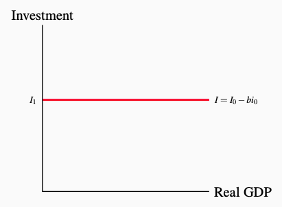
Figure 6.5: The Investment Function Planned investment expenditure is independent of current GDP. A change in the interest rate would shift the line.

Investment, unlike consumption, is a volatile component of expenditure. Changes in business expectations about future markets and profits happen frequently. New technologies and products, like hybrid automobiles, “clean” diesel engines, biofuels, LED televisions, advanced medical diagnostic processes, renewable energy products and “green” building materials lead to the investment in factories to produce these products and the infrastructure to use them. Investment expenditures increase. A sudden uncertainty about safety reduces demand for plastic products in food and beverage packaging. Investment in new capacity to produce these products drops and a search for new packaging begins. Increased gasoline prices reduce the demand for large cars and trucks, leading some auto manufacturers to close plants and cut investment spending. More recently, sharp drops in prices for conventional energy and difficult financial market conditions have led to the postponement and cancellation of large investments in both conventional and alternative energy projects.

Fluctuations in investment in Canada caused by these and other factors are illustrated in Figure 6.6. The steep drop in investment expenditure in 2008 and 2009 is of particular note. This was a major cause of the recession that followed the financial crisis of 2009. The coincident drop in exports also contributed to that recession. Volatility in these expenditure components over the period covered by Figure 6.6 are major causes of business cycles in Canadian real GDP and employment.

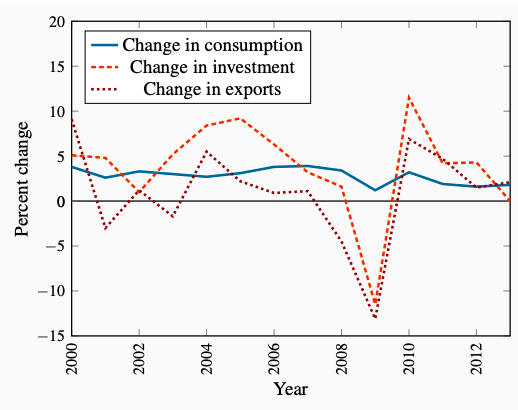
Figure 6.6: Annual Percent Change in Real Consumption, Investment and Exports, Canada 2000-2013 Source: Statistics Canada, CANSIM Table 380-0064

---

¹The Greek letter ∆ (Delta) means ‘change in’. For example, ∆C means ‘change in C’.