2.2: Variables, Data and Index Numbers

Economic theories and models are concerned with economic variables. Variables are measures that can take on different sizes. The interest rate on a student loan, for example, is a variable with a certain value at a point in time but perhaps a different value at an earlier or later date. Economic theories and models explain the causal relationships between variables.

Variables: measures that can take on different values.

Data are the recorded values of variables. Sets of data provide specific values for the variables we want to study and analyze. Knowing that the Don Valley Parkway is congested does not tell us how slow our trip to downtown Toronto will be. To choose the best route downtown we need to ascertain the degree of congestion—the data on traffic density and flow on alternative routes. A model is useful because it defines the variables that are most important and to the analysis of travel time and the data that are required for that analysis.

Data: recorded values of variables.

Sets of data also help us to test our models or theories, but first we need to pay attention to the economic logic involved in observations and modelling. For example, if sunspots or baggy pants were found to be correlated with economic expansion, would we consider these events a coincidence or a key to understanding economic growth? The observation is based on facts or data but it need not have any economic content. The economist’s task is to distinguish between coincidence and economic causation.

While the more frequent wearing of loose clothing in the past may have been associated with economic growth because they both occurred at the same time (correlation), one could not argue on a logical basis that this behaviour causes good economic times. Therefore, the past association of these variables should be considered as no more than a coincidence.

Once specified on the basis of economic logic, a model must be tested to determine its usefulness in explaining observed economic events. The earlier example of a model of house prices and mortgage rates was based on the economics of the effect of financing cost on expenditure and prices. But we did not test that model by confronting it with the data. It may be that effects of mortgages rates are insignificant compared to other influences on house prices.

Time-Series Data

Data come in several forms. One form is time-series, which reflects a set of measurements made in sequence at different points in time. Table 2.1 reports the annual time series values for several price series. Such information may also be presented in charts or graphs. Figure 2.1 plots the data from column 2, and each point represents the data observed for a specific time period. The horizontal axis reflects time in years, the vertical axis price in dollars.

Time-series: a set of measurements made sequentially at different points in time.

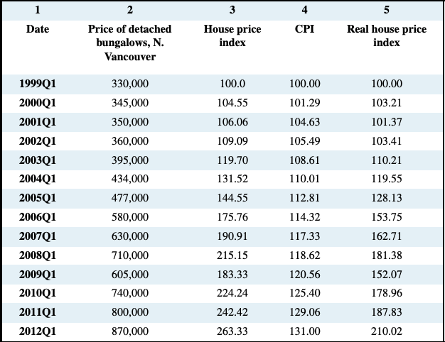
Table 2.1: House Prices and Price Indexes
Source: Prices for North Vancouver houses come from Royal Le Page; CPI
from Statistics Canada, CANSIM II, V41692930 and author’s calculations.

Annual data report one observation per year. We could, alternatively, have presented them in quarterly, monthly, or even weekly form. The frequency we use depends on the purpose: If we are interested in the longer-term trend in house prices, then the annual form suffices. In contrast, financial economists, who study the behaviour of stock prices, might not be content with daily or even hourly prices; they may need prices minute-by-minute. Such data are called high-frequency data, whereas annual data are low-frequency data.

High (low) frequency data: series with short (long) intervals between observations.

When data are presented in charts or when using diagrams the scales on the axes have important visual effects. Different scales on either or both axes alter the perception of patterns in the data. To illustrate this, the data from columns 1 and 2 of Table 2.1 are plotted in Figures 2.2 and 2.3, but with a change in the scale of the vertical axis.

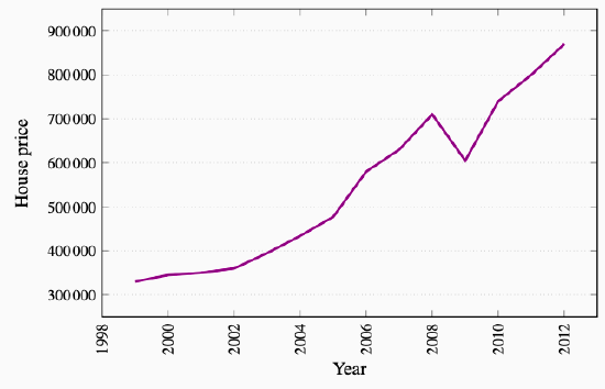
Figure 2.2: House Prices in Dollars North Vancouver 1999-2012

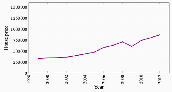
Figure 2.3: House Prices in Dollars North Vancouver 1999-2012

Cross-Section Data

In contrast to time-series data, cross-section data record the values of different variables at a point in time. Table 2.2 contains a cross-section of unemployment rates for Canada and Canadian provinces economies. For January 2012 we have a snapshot of the provincial economies at that point in time, likewise for the months until June. This table therefore contains repeated cross-sections.

When the unit of observation is the same over time such repeated cross sections are called longitudinal data. For example, a health survey that followed and interviewed the same individuals over time would yield longitudinal data. If the individuals differ each time the survey is conducted, the data are repeated cross sections. Longitudinal data therefore follow the same units of observation through time.

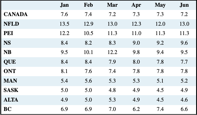
Table 2.2: Unemployment Rates, Canada and Provinces, Month 2012, Seasonally Adjusted
Source: Statistics Canada CANSIM Table 282-0087

Cross-section data: values for different variables recorded at a point in time.

Repeated cross-section data: cross-section data recorded at regular or irregular intervals.

Longitudinal data: follow the same units of observation through time.

Index Numbers

It is important in economic analysis to discuss and interpret data in a meaningful manner. Index numbers help us greatly in doing this. They are values of a given variable, or an average of a set of variables expressed relative to a base value. The key characteristics of indexes are that they are not dependent upon the units of measurement of the data in question, and they are interpretable easily with reference to a given base value. To illustrate, let us change the price data in column 2 of Table 2.1 into index number form.

Index number: value for a variable, or an average of a set of variables, expressed relative to a given base value.

The first step is to choose a base year as a reference point. This could be any one of the periods. We will simply take the first period as the year and set the price index value equal to 100 in that year. The value of 100 is usually chosen in order to make comparisons simple, but in some cases a base year value of 1.0 is used. If the base year value of 100 is used, the value of index in any year t is:

\[\text{Value of index} = \frac {\text{Absolute value in year} \,t} {\text{Absolute value in base year}} \:\times\:100\]

Suppose we choose 1999 as the base year for constructing an index of the house prices given in Table 2.1 House prices in that year were $330,000. Then the index for the base year has a value:

\(\text{Index in} \:1999 = \displaystyle\frac {$330,000} {$330,000} \times \:100 = \:100\)

Applying the method to each value in column 2 yields column 3, which is now in index number form. For example, the January 2003 value is:

\(\text{Index in} \:2003 = \displaystyle\frac {$395,000} {$330,000} \times \:100 = \:119.7\)

Each value in the index is interpreted relative to the value of 100, the base price in January 1999. The beauty of this column lies first in its ease of interpretation. For example, by 2003 the price increased to 119.7 points relative to a value of 100. This yields an immediate interpretation: The index has increased by 19.7 points per hundred or percent. While it is particularly easy to compute a percentage change in a data series when the base value is 100, it is not necessary that the reference point have a value of 100. By definition, a percentage change is given by the change in values relative to the initial value, multiplied by 100. For example, the percentage change in the price from 2006 to 2007, using the price index is: (190.91−175.76)/175.76×100 = 8.6 percent.

Percentage change = (change in values) / original value × 100.

Furthermore, index numbers enable us to make comparisons with the price patterns for other goods much more easily. If we had constructed a price index for wireless phones, which also had a base value of 100 in 1999, we could make immediate comparisons without having to compare one set of numbers defined in dollars with another defined in tens of thousands of dollars. In short, index numbers simplify the interpretation of data.

Composite Index Numbers

Index numbers have even wider uses than those we have just described. Suppose you are interested in the price trends for all fuels as a group in Canada during the last decade. You know that this group includes coal, natural gas, and oil, but you suspect that these components have not all been rising in price at the same rate. You also know that, while these fuels are critical to the economy, some play a bigger role than others, and therefore should be given more importance, or weight, in a general fuel price index. In fact, the official price index for these fuels is a weighted average of the component price indexes. The fuels that are more important get a heavier weighting in the overall index. For example, if oil accounts for 60 percent of fuel use, natural gas for 25 percent, and coal for 15 percent, the price index for fuel could be computed as follows:

\[\text{Fuel price index} = (\text{oil index} \times \,0.6) + (\text{natural gas index} \times \,0.25) + (\text{coal index} \times \,0.15)\]

To illustrate this, Figure 2.4 presents the price trends for these three fuels. The data come from Statistics Canada’s CANSIM database. In addition, the overall fuel price index is plotted. It is frequently the case that components do not display similar patterns, and in this instance the composite index follows oil most closely, reflecting the fact that oil has the largest weight.

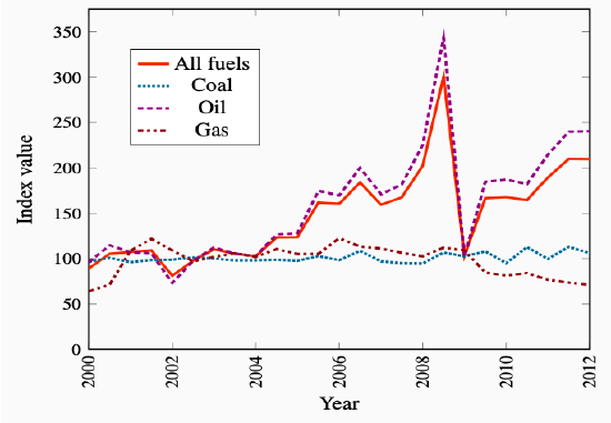
Figure 2.4: Composite Fuel Price Index
Source: Statistics Canada. Table 330-0007 – Raw materials price indexes,
monthly (index, 2002=100), CANSIM.

Other Composite Price Indexes

The fuels price index is just one of many indexes constructed to measure a composite group of economic variables. There are also published indexes of commodity prices, including and excluding fuels, agricultural prices, average hourly earnings, industrial production, unit labour costs, Canadian dollar effective exchange rate (CERI), the S&P/TSX stock market prices and consumer prices to list just a few. All these indexes are designed to reduce the complexity of the data on key sectors of the economy and important economic conditions.

The consumer price index (CPI) is the most widely quoted price index in the economy. It measures the average price level in the economy and changes in the CPI provide measures of the rate at which consumer goods and services change in price—inflation if prices increase, deflation if prices decline.

The CPI is constructed in two stages. First, a consumer expenditure survey is use to establish the importance or weight of each of eight categories in a ‘basket’ of goods and services. Then the cost of this basket of services in a particular year is compared to its cost in the chosen base year. With this base year cost of the basket set at 100 the ratio of the cost of the same basket in any other year to its cost in the base year multiplied my 100 gives the CPI for that year. The CPI for any given year is:

\[CPI_t = \frac {\text{Cost of basket in year}\:t}{\text{Cost of basket in base year}} \times \:100\]

Consumer price index: the average price level for consumer goods and services

Inflation rate: the annual percentage increase in the consumer price index

Deflation rate: the annual percentage decrease in the consumer price index

Using price indexes

The CPI is useful both as an indicator of how much prices change in the aggregate, and also as an indicator of relative price changes. Column 4 of Table 2.1 provides the Vancouver CPI with the same base year as the North Vancouver house price index. Note how the two indexes move very differently over time. The price of housing has increased considerably relative to the overall level of prices in the local economy, as measured by the CPI: Housing has experienced a relative price increase, or a real price index. This real increase is to be distinguished from the nominal price index, which is measured without reference to overall prices. The real price index for housing (or any other specific product) is obtained by dividing its specific price index by the CPI.

\[\text{Real house price index} = \frac {\text{nominal house price index}}{CPI} \:\times \:100\]

Real price index: a nominal price index divided by the consumer price index, scaled by 100.

Nominal price index: the current dollar price of a good or service.

The resulting index is given in column 5 of Table 2.1. This index has a simple interpretation: It tells us by how much the price of Vancouver houses has changed relative to the general level of prices for goods and services. For example, between 1999 and 2004 the number 119.55 in column 5 for the year 2004 indicates that housing increased in price by 19.55 percent relative to prices in general.

Here is a further simple example. Table 2.3 reports recent annual data on indexes of nominal earnings, measured in current dollars, both average weekly and hourly rates, over the 2003-2011 time period. The table also reports the consumer price index for the same time period. To simplify the illustration all indexes have been re-based to 2003=100 by dividing the reported value of the index in each year by its value in 2003 and multiplying by 100.

The table shows the difference between changes in nominal and real earnings. Real earnings are measured in constant dollars adjusted for changes in the general price level. The adjustment is made by dividing the indexes of nominal earnings in each year by the consumer price index in that year and multiplying by 100.

Nominal earnings: earnings measured in current dollars.

Real earnings: earnings measure in constant dollars to adjust for changes in the general price level.

As measured by the nominal weekly and hourly indexes, nominal earnings increased by 26 to 27 percent over the eight year period 2003-2011. However, the general price level as measured by the consumer price index (CPI) increased by close to 17 percent over the same period. As a result, real earnings, measured in terms of the purchasing power of nominal earnings increased by only about 9 percent, notable less than in 26 percent increase in nominal earnings.

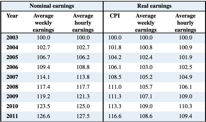
Table 2.3: Nominal and Real Earnings in Canada 2003-2011
Source: Statistics Canada, CANSIM Series V1558664, V1606080 and
V41690914 and author’s calculations

These observations illustrate two important points. First the distinction between real and nominal values is very important. If the general price level is changing, changes in real values will differ from changes in nominal values. Real values change by either less or more than changes in nominal values. Second, in addition to tracking change over time, index numbers used in combination simplify the adjustment from nominal to real values, as shown in both Table 2.1 and 2.3.

However, a word of caution is necessary. Index numbers can be used to track both nominal and real values over time but they do not automatically adjust for change in the quality of products and services or the changing patterns of output and use in the cases of composite indexes. Index number bases and weights need constant adjustment to deal with these issues.