6.4: Aggregate Expenditure and Equilibrium Output in the Short Run

Aggregate expenditure is planned expenditure by firms and households on currently produced final goods and services at each level of current national income. The aggregate expenditure function (AE) is the relationship between planned expenditure in the total economy and real national income or GDP. Table 6.2 and Figure 6.8 together show the aggregate expenditure function in terms of numerical examples and diagrams.

Aggregate expenditure function (AE): the relationship between planned expenditure in the total economy and real national income or GDP.

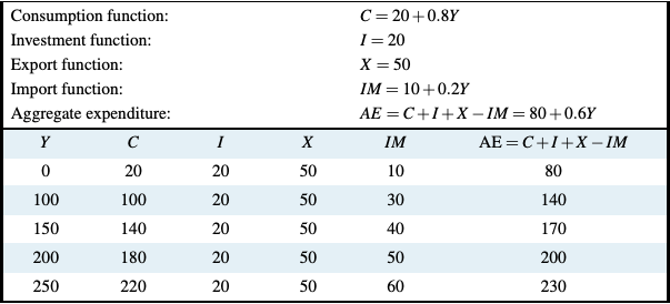
Table 6.2: The Aggregate Expenditure Function: A Numerical Example

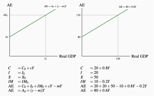
Figure 6.8: Aggregate Expenditure

Aggregate expenditure AE, as defined above and earlier by Equation 6.1, is:

\(\text{AE} = C + I + X - IM\)

In Table 6.2 and Figure 6.8, the aggregate expenditure function is derived using this equation. Aggregate expenditure is different at different income levels because of induced expenditure on consumption and imports. Aggregate expenditure changes by (c − m) times any change in income. (∆AE = ∆C − ∆IM = c∆Y − m∆Y). In the Figure the vertical intercept of AE is the sum of autonomous expenditure. The slope of AE is (c − m), the marginal propensity to consume minus the marginal propensity to import.

Many things other than income influence autonomous expenditure. It is not fixed, but it is independent of income. The AE function separates the change in expenditure directly induced by changes in income from changes caused by other sources. All other sources of changes in aggregate expenditure are shown as shifts of the AE line. If firms get more optimistic about future demand and profit and invest more, autonomous expenditure rises. The new AE line is parallel to, but higher than, the old AE line. A financial crisis like that in the US in 2008 or the ongoing sovereign debt crisis in Europe shifts the AE line down. A change in exports shifts the AE line up or down without changing its slope as exports either increase or decrease.

Equilibrium Output

Output is said to be in short-run equilibrium when planned aggregate expenditure (AE) equals the current output of goods and services (Y). Spending plans are not frustrated by a shortage of goods and services. Nor do business firms make more output than they can sell. In short-run equilibrium, output equals the total of goods and services that households, businesses, and residents of other countries want to buy. Real GDP is determined by aggregate expenditure.

Short-run equilibrium output: Aggregate expenditure equals current output.

In Figure 6.9 real GDP is measured on the horizontal axis and aggregate spending on the vertical axis. The 45° line labeled \(Y = \text{AE}\), illustrates the equilibrium condition. At every point on the line, AE measured on the vertical axis equals current output, Y, measured on the horizontal axis. This 45° line has a slope of 1.

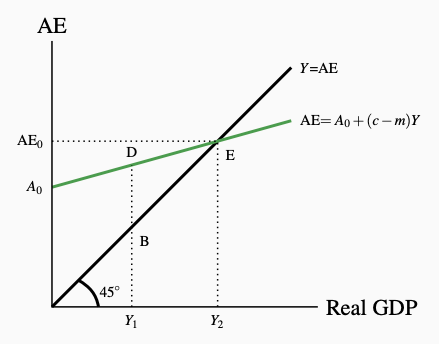
Figure 6.9: The 45° Diagram and Equilibrium GDP
The 45° line gives Y = AE the equilibrium condition. At point E the AE line
crosses the 45° line and AE₀ = Y₂. This is the equilibrium. At Y₁, AE > Y
and unplanned reductions in inventories provide the incentive to increase Y.

The AE function in Figure 6.9 starts from a positive intercept on the vertical axis to show autonomous aggregate expenditure, and has a slope which is less than one and equal to (c − m). This positive intercept and slope less than 1 means that the AE line crosses the 45° line at E. On the 45° line, the value of output (and income) on the horizontal axis equals the value of expenditure on the vertical axis, as required by the national accounts framework. Since E is the only point on the AE line also on the 45° line, it is the only point at which output and planned expenditure are equal. It is the equilibrium point.

This is the only aggregate expenditure that just buys all current output. For example, assume as shown in the diagram, that output and incomes are only Y₁. Aggregate expenditure at D is not equal to output as measured at B. Planned expenditure is greater than current output. Aggregate spending plans cannot all be fulfilled at this current output level. Consumption and export plans will be realized only if business fails to meet its investment plans as a result of an unplanned fall in inventories of goods.

In Figure 6.9 all outputs less than the equilibrium output Y₂, are too low to satisfy planned aggregate expenditure. The AE line is above the 45° line along which expenditure and output are equal. Conversely, if real GDP is greater than Y₂ aggregate expenditure is not high enough to buy all current output produced. Businesses have unwanted and unplanned increases in inventories of unsold goods.

We can also find equilibrium output using the consumption function (Equation 6.2), the investment function (Equation 6.4), the export function (Equation 6.5), the import function (Equation 6.6), and the equilibrium condition Y =AE. We have:

\(\text{AE} = C + I + X - IM\)

\(C = C_0 + CY\)

\(I = I_0\)

\(X = X_0\)

\(IM = IM_0 + mY\)

Using the equilibrium condition Y = AE and solving for Y gives:

\(\begin{align*} Y &= C + I + X - IM \\
Y &= C_0 + cY + I_0 + X_0 - IM_0 - mY \\
Y - cY + mY &= C_0 + I_0 + X_0 - IM_0 \\
Y(1- c + m) &= C_0 + I_0 + X_0 - IM_0 \end{align*}\)

This gives:

\[Y_e = \displaystyle\frac {(C_0 + I_0 + X_0 - IM_0)}{(1 - c + m)} = \displaystyle\frac {A_0}{1 - c + m}\]

This is the equilibrium output Y₂ we found using the diagram in Figure 6.9. From the numerical example in Table 6.2 we have:

\(\begin{align*} C &= 20 + 0.8Y \\
I &= 20 \\
X &= 50 \\
IM &= 10 + 0.2Y \\
AE &= 20 + 0.8Y + 20 + 50 - 10 - 0.2Y \\
AE &= 80 + 0.6Y \end{align*}\)

Using the equilibrium condition Y =AE and solving for Y gives:

\(\begin{align*} Y &= 80 + 0.6Y \\
Y &= 0.6Y = 80 \\
Y &= \displaystyle\frac {80}{(1 - 0.6} \\
Y_2 &= 200 \end{align*}\)

When we look back at Table 6.2 we do see that aggregate expenditure and income are equal when income is 200. You can construct a diagram like Figure 6.9 using the numerical values for aggregate expenditure in Table 6.2 and a 45° line to show equilibrium Y_e = 200.

Adjustment Towards Equilibrium

Unplanned changes in business inventories cause adjustments in output that move the economy to equilibrium output. Suppose in Figure 6.9 the economy begins with an output Y₁, below equilibrium output Y_e. Aggregate expenditure is greater than output Y₁. If firms have inventories from previous production, they can sell more than they have produced by running down inventories for a while. Note that this fall in inventories is unplanned. Planned changes in inventories are already included in planned investment and aggregate expenditure.

If firms cannot meet planned aggregate expenditure by unplanned inventory reductions, they must turn away customers. Either response—unplanned inventory reductions or turning away customers— is a signal to firms that aggregate expenditure is greater than current output, markets are strong, and output and sales can be increased profitably. Hence, at any output below Y_e, aggregate expenditure exceeds output and firms get signals from unwanted inventory reductions to raise output.

Conversely, if output is initially above the equilibrium level, Figure 6.9 shows that output will exceed aggregate expenditure. Producers cannot sell all their current output. Unplanned and unwanted additions to inventories result, and firms respond by cutting output. In recent years, North American auto producers found demand for their cars and trucks was less than they expected. Inventories of new cars and trucks built up on factory and dealer lots. Producers responded by lowering production to try to reduce excess inventory. In general terms, when the economy is producing more than current aggregate expenditure, unwanted inventories build up and output is cut back.

Hence, when output is below the equilibrium level, firms raise output. When output is above the equilibrium level, firms reduce output. At the equilibrium output Y_e, firms sell their current output and there are no unplanned changes to their inventories. Firms have no incentive to change output.

Equilibrium Output and Employment

In the examples of short-run equilibrium we have discussed, output is at Y_e with output equal to planned expenditure. Firms sell all they produce, and households and firms buy all they plan to buy. But it is important to note that nothing guarantees that equilibrium output Y_e is the level of potential output Y_p. When wages and prices are fixed, the economy can end up at a short-run equilibrium below potential output with no forces present to move output to potential output. Furthermore, we know that, when output is below potential output, employment is less than full and the unemployment rate u is higher than the natural rate u_n. The economy is in recession and by our current assumptions neither price flexibility nor government policy action can affect these conditions.