4. Data Analysis

Last updated
Save as PDF

Page ID: 38381

$ \newcommand{\vecs}[1]{\overset { \scriptstyle \rightharpoonup} {\mathbf{#1}} } $ $ \newcommand{\vecd}[1]{\overset{-\!-\!\rightharpoonup}{\vphantom{a}\smash {#1}}} $$\newcommand{\id}{\mathrm{id}}$ $ \newcommand{\Span}{\mathrm{span}}$ $ \newcommand{\kernel}{\mathrm{null}\,}$ $ \newcommand{\range}{\mathrm{range}\,}$ $ \newcommand{\RealPart}{\mathrm{Re}}$ $ \newcommand{\ImaginaryPart}{\mathrm{Im}}$ $ \newcommand{\Argument}{\mathrm{Arg}}$ $ \newcommand{\norm}[1]{\| #1 \|}$ $ \newcommand{\inner}[2]{\langle #1, #2 \rangle}$ $ \newcommand{\Span}{\mathrm{span}}$ $\newcommand{\id}{\mathrm{id}}$ $ \newcommand{\Span}{\mathrm{span}}$ $ \newcommand{\kernel}{\mathrm{null}\,}$ $ \newcommand{\range}{\mathrm{range}\,}$ $ \newcommand{\RealPart}{\mathrm{Re}}$ $ \newcommand{\ImaginaryPart}{\mathrm{Im}}$ $ \newcommand{\Argument}{\mathrm{Arg}}$ $ \newcommand{\norm}[1]{\| #1 \|}$ $ \newcommand{\inner}[2]{\langle #1, #2 \rangle}$ $ \newcommand{\Span}{\mathrm{span}}$$\newcommand{\AA}{\unicode[.8,0]{x212B}}$

You've designed your experiment, collected your data, and cleaned it, what next? Analysis! In this section we will go over how to perform t-tests, ANOVA, and correlations/linear regression in R. Instructions for how to find descriptive statistics can be found in the previous section Data Cleaning with the summarise() function.

T-test

Below we will outline the basics for one-sample, paired, and independent t-tests with example output using the mtcars dataset.

One-Sample

For a one-sample t-test, we use the following code where y is the name of your variable of interest and mu is set equal to the mean specified in the null hypothesis.

t.test(y, mu = 0)

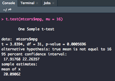
Screen Shot 2019-12-10 at 1.43.54 PM.png

As you can see, the output very clearly states what the t-value, degrees of freedom, and p-value are.

Tip

To pull a specific row from a dataset to use as a variable of interest, use the $ operator. For example if we wanted to use the mpg variable from the mtcars dataset, we would write mtcars$mpg in the command.

Paired-Sample

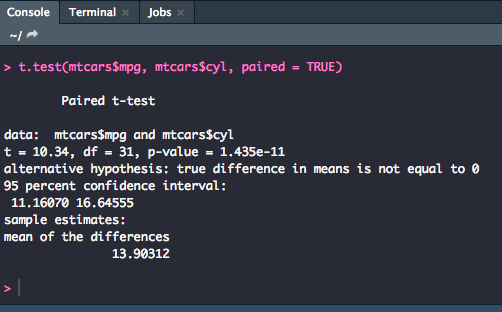
For a paired-sample t-test, you will use two variables (which should be vectors of data), y1 and y2, or one vector of data and a grouping variable.

Definition

A grouping variable sorts data within data files into categories or groups.

Ex. Sorting male and female participants as male = 0 and female = 1 in a vector.

t.test(y1, y2, paired = TRUE)

Independent

For an independent t-test, you will use much the same syntax with a few minor adjustments.

t.test(y1, y2, paired = FALSE)

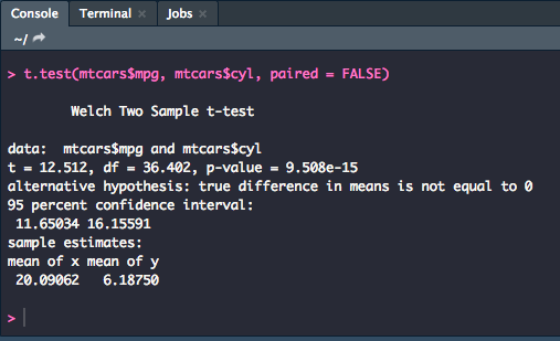
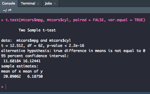
Screen Shot 2019-12-10 at 1.46.06 PM.png

R will assume that the variances of the two variables are unequal and will default to Welch's test. To switch the assumption use the following syntax:

t.test(y1, y2, paired = FALSE, var.equal = TRUE)

ANOVA

Below we will outline how to conduct a one-way ANOVA, the Tukey HSD post-hoc test, and a two-way ANOVA.

One-Way

Previously, we discussed how to make objects in the global environment using the <- operator. Throughout this section, it has been assumed that the data being used is just an object already loaded straight from a .csv file. With ANOVA, there are some extra manipulations that have to be made to the data.

First, you will want to create a new object that converts the variable which contains the factor specifications to an ordered level.

mtcars.anova <- mtcars %>%
  mutate(cyl = factor(cyl, ordered = TRUE))

Above, we have created the new mtcars.anova object in the global environment. Within the mtcars.anova set, the cyl column has been mutated (changed) to be, instead, designating ordered levels assuming that the different levels of analysis will be based on how many cylinders a car has. For the purpose of this example, we will be running it against mpg as the dependent variable.

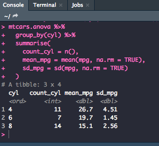
Next, you will compute the mean and standard deviation using the following code:

mtcars.anova %>%
    group_by(cyl) %>%
    summarise(
            count_cyl = n(),
            mean_mpg = mean(mpg, na.rm = TRUE),
            sd_mpg = sd(mpg, na.rm = TRUE)
         )

Screen Shot 2019-12-26 at 1.26.33 PM.png

While it isn't necessary, it always a good idea to create a visualization to check for differences in distribution. The best way to visualize is to use ggplot. The following is code for a basic box plot with ggplot.

ggplot(mtcars.anova, aes(x = cyl, y = mpg, fill = cyl)) +
    geom_boxplot() +
    geom_jitter(shape = 15,
        color = "steel blue",
        position = position_jitter(0.21)) +
    theme_classic()

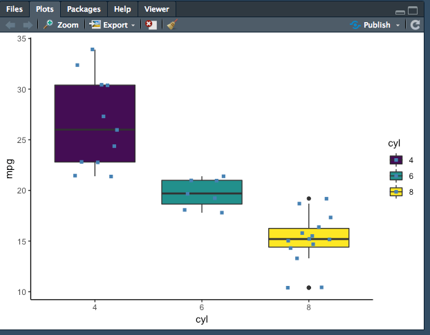
Screen Shot 2019-12-26 at 1.34.21 PM.png

The graph does show quite the difference in distribution. For more information on how to create any graph you would like, visit http://r-statistics.co/ggplot2-Tutorial-With-R.html

To perform a one way ANOVA on this dataset, you will want to save the model (aov) as an object in the global environment, so use the following syntax to run the model. Then, using the summary() function you will be able to get the output you need.

anova_one_way <- aov(mpg~cyl, data = mtcars.anova)
summary(anova_one_way)

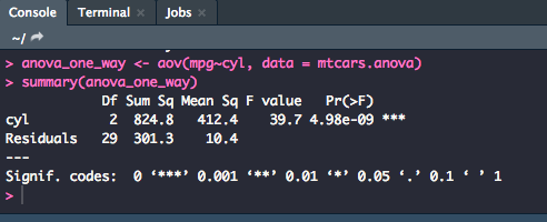
Screen Shot 2019-12-26 at 1.43.59 PM.png

From this output, you can say that there is a significant difference between number of cylinders a car has and its miles per gallon [F(2,29) = 39.7, p = .000]

Significance levels can either be pulled directly from the Pr(>F) column or taken from the significance code next to the p-value which can be translated with the codes at the bottom of the output. For example, in the output above, the *** code would be a p-value of .000.

Pairwise Comparison

With running an ANOVA, you will often want to run pairwise comparisons to prevent making a Type I error. A common way to do so is to use the Tukey Honestly Significant Difference test or Tukey HSD.

TukeyHSD(anova_one_way)

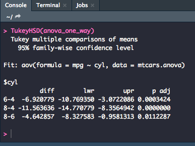
Screen Shot 2019-12-26 at 2.11.53 PM.png

For these results, you could summarize that the Tukey pairwise comparison (or post-hoc text) showed that the 6-cylinder group differed significantly from the 4-cylinder and the 8-cylinder groups (p < .001, p < .05) and the 4-cylinder group also differed significantly from the 8-cylinder group (p = .000).

Two-Way

The last ANOVA we will discuss in this section is how to run a two-way ANOVA. The process would be similar to that of the one-way ANOVA but would differ slightly in the final code for running the ANOVA model. For the purposes of this example, we will continue to use the mtcars.anova dataset that we made previously, pulling the cyl and mpg variables as before along with disp (displacement).

anova_two_way <- aov(mpg~cyl + disp, data = mtcars.anova)
summary(anova_two_way)

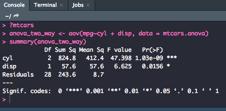
Screen Shot 2019-12-26 at 2.35.11 PM.png

The table reads exactly as the one-way ANOVA did, just with a second row with the statistics for disp.

Correlation and Linear Regression

Our final types of analysis covered in this section will be correlation and linear regression models.

Pearson Correlation

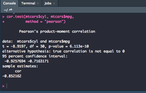
A common way to run a correlation test between two variables is to use the Pearson Correlation. For example, to find the correlation between cyl and mpg, use the following code:

cor.test(mtcars$cyl, mtcars$mpg, 
         method = "pearson")

Screen Shot 2019-12-26 at 3.15.22 PM.png

Note

In this model, we used the $ operator to pull a column from the mtcars dataset. Using the pipe, %>%, doesn't always work, so when in a situation when you need to pull directly from a dataset, you can do so by connecting the dataset you're pulling from and which coulmn you want: data$column

Linear Regression

If you want to find predictions instead of correlations, you would use linear regression. You would then designate one variable as the predictor and one as the outcome. For this example, cyl will be the predictor and mpg will be the outcome variable. Like for the ANOVA, you will want to create an object for the model in the global environment.

linearMod <- lm(mpg~cyl, data = mtcars)
summary(linearMod)

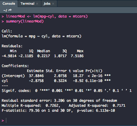
Screen Shot 2019-12-26 at 3.26.31 PM.png

According to the output above, there was a significant effect of number of cylinders on miles per gallon [F(1,30) = 79.56, p = .000, R2 = 0.73]. The F statistic values come from the very bottom line of the output, and the R2 value is from the "Multiple R-squared" line.

You can also do multiple regressions. For example, let's see if cyl, wt, and carb have an effect on mpg.

linearMod <- lm(mpg~cyl + wt + carb, data = mtcars)
summary(linearMod)

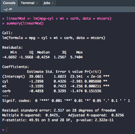
Screen Shot 2019-12-26 at 3.44.59 PM.png

This output reads exactly the same as the previous, only with more coefficient rows because we used more variables. For reporting individual t-values and p-values with the linear regression model, use the values from the t value and Pr(>|t|) columns. For example, the individual predictor of weight on miles per gallon was significant (t = -4.256, p = .000).