7.6: The Public Debt and the Budget Balance

Last updated
Save as PDF

Page ID: 11828

$ \newcommand{\vecs}[1]{\overset { \scriptstyle \rightharpoonup} {\mathbf{#1}} } $ $ \newcommand{\vecd}[1]{\overset{-\!-\!\rightharpoonup}{\vphantom{a}\smash {#1}}} $$\newcommand{\id}{\mathrm{id}}$ $ \newcommand{\Span}{\mathrm{span}}$ $ \newcommand{\kernel}{\mathrm{null}\,}$ $ \newcommand{\range}{\mathrm{range}\,}$ $ \newcommand{\RealPart}{\mathrm{Re}}$ $ \newcommand{\ImaginaryPart}{\mathrm{Im}}$ $ \newcommand{\Argument}{\mathrm{Arg}}$ $ \newcommand{\norm}[1]{\| #1 \|}$ $ \newcommand{\inner}[2]{\langle #1, #2 \rangle}$ $ \newcommand{\Span}{\mathrm{span}}$ $\newcommand{\id}{\mathrm{id}}$ $ \newcommand{\Span}{\mathrm{span}}$ $ \newcommand{\kernel}{\mathrm{null}\,}$ $ \newcommand{\range}{\mathrm{range}\,}$ $ \newcommand{\RealPart}{\mathrm{Re}}$ $ \newcommand{\ImaginaryPart}{\mathrm{Im}}$ $ \newcommand{\Argument}{\mathrm{Arg}}$ $ \newcommand{\norm}[1]{\| #1 \|}$ $ \newcommand{\inner}[2]{\langle #1, #2 \rangle}$ $ \newcommand{\Span}{\mathrm{span}}$$\newcommand{\AA}{\unicode[.8,0]{x212B}}$

Budget balances and outstanding debt are closely related. A student’s debt at the time of graduation is the sum of her budget balances during years of study. In any year in which her income is less than her expenses, she finances the difference by borrowing. In another year, if income is greater than expenses, she can repay some previous borrowing. In the end, the sum of borrowings minus the sum of repayments is her outstanding student debt (loan). This debt is a result of borrowing to finance investment in education.

Similarly, the outstanding public debt (PD) at any point in time is simply the sum of past government budget balances. Governments borrow to finance budget deficits by selling government bonds to households and businesses. Budget surpluses reduce the government’s financing requirements. Some bonds previously issued mature without being refinanced. In simple terms, the budget balance in any year changes the outstanding public debt by an equal amount but with the opposite sign. A positive balance, a surplus (BB > 0), reduces the public debt (∆PD < 0). A negative balance, a deficit (BB < 0), increases the public debt (∆PD > 0). Using PD to represent the outstanding public debt, we can express the link between the public debt and the government’s budget balance as:

\[\Delta PD = -BB\]

Public debt (PD): the outstanding stock of government bonds issued to finance government budget deficits.

Figures 7.8 and 7.9 show the relationship between the government budget balance and the change in the public debt relative to GDP based on Canadian data for the 1988-2012 period. Recognizing that growth in the economy makes absolute numbers for deficits and debt hard to evaluate, the budget balance and the change public debt are presented as percentages of nominal GDP. The effects of budget balances on the public debt are illustrated clearly in the diagrams.

Screenshot 2019-05-18 at 01.27.40.png

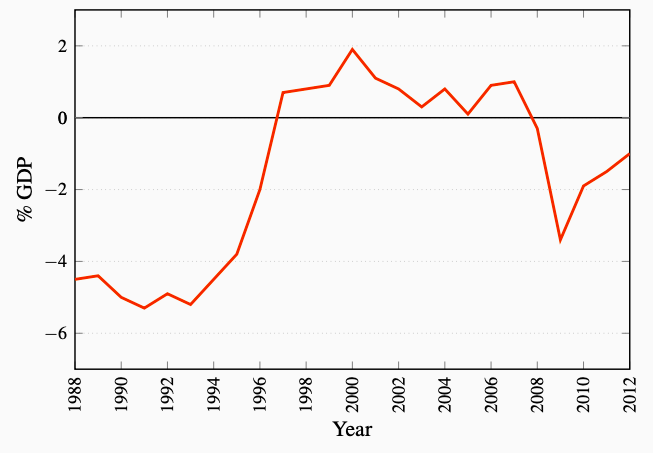
Figure 7.8: Canadian Federal Government BB % GDP
Source: Department of Finance, Fiscal Reference Tables (2013)

Screenshot 2019-05-18 at 01.28.52.png

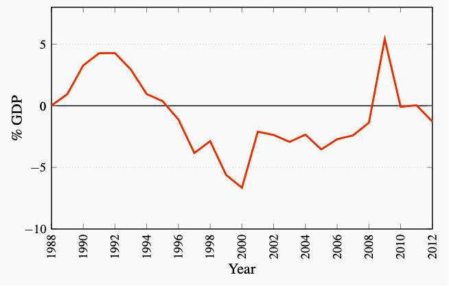
Figure 7.9: Change in Federal Government Public Debt Ratio
Source: Department of Finance, Fiscal Reference Tables 2013. Bank of
Canada, Banking and Financial Statistics Feb 2014 and author's calcula-
tions.

In the years from 1995 to 2007 the Government of Canada had budget surpluses. Things were different in the years before 1995. Large budget deficits, averaging more than 5 percent of GDP, were the norm in the late 1980s and early 1990s. As a result, the outstanding federal government public debt increased, and increased faster than GDP, pushing the ratio of public debt to GDP up from 38 percent of GDP in 1983 to 68 percent of GDP in 1996. The cost of the interest payments the government had to make to the holders of its bonds increased from $3.9 billion to $42.4 billion. These costs accounted for almost 30 percent of budgetary expenses in 1995.

As a result, Canadian fiscal and budgetary policy shifted in 1995 to focus much more on deficit and debt control than on income stabilization. As Figure 7.8 shows, the federal budget was in surplus from 1997 until 2007. This reduced the debt to GDP ratio each year until 2008 as in Figure 7.9.

The financial crisis and recession of 2008-2009 and the federal government’s Economic Action Plan changed this focus and pattern of fiscal policy. Fiscal stimulus through increased government expenditures and modest tax credits together with the recession in income created budget deficits in 2008-2013. These deficits added directly to the federal government debt. Larger debt combined with little or no growth in nominal GDP in 2009 and 2010 caused a sharp increase in the debt ratio shown in Figure 7.9. The focus of Federal Budget plans for recent years, as the recovery from recession seems to be underway, has shifted back to budget deficit control and reduction and a return to lower public debt ratios.

Although cumulative deficits can raise the public debt dramatically, it is not the absolute value of the outstanding debt that should be of interest or concern. If, at the same time as the debt is rising, the economy is growing and tax revenues are rising as a result of a growing tax base, the government may be able to service a growing debt without having to raise taxes. The public debt ratio (PD/Y) is then the appropriate measure of the debt situation. A rise in the outstanding debt is not in itself a source of concern. However, the government cannot allow the debt ratio to rise without limit.

Public debt ratio (PD/Y): the ratio of outstanding government debt to GDP.

Recent sovereign debt crises in Portugal, Ireland, Greece and Spain provide clear examples of the difficulties high and rising public debt ratios cause. In those countries and others in Europe, and in the US, the government costs of rescuing banks in financial distress after 2008 combined in many cases with already large budget deficits, compounded by the recession in economic growth raised public debt ratios sharply. Table 7.2 shows the early stages of these increases in from 2007 to 2012. The consequence was a loss of financial market confidence in the ability of some of these countries to pay interest on and subsequently retire outstanding government bonds, let alone service new bond issues to finance current deficits. Interest rates for new bond issues increased sharply and Greece and Ireland needed financial bailouts from joint EU rescue funds. This has provided time for fiscal adjustment but the economic growth required to solve sovereign debt issues remains elusive.

We will return to the relationship between fiscal policy and the public debt and examine the dynamics of the public debt ratio in Chapter 12.

This completes our introduction to the government budget, fiscal policy, aggregate expenditure, and the economy. We have seen two ways in which the government sector affects aggregate expenditure and output. Government expenditure is a part of autonomous aggregate expenditure. It affects the position of the AE function, equilibrium output, and the aggregate demand curve. The net tax rate is a leakage from the income expenditure flow. It affects induced expenditure, the slope of the AE function, the size of the multiplier, equilibrium output, and the AD curve. Government expenditure and the net tax rate are policy levers the government can use to influence aggregate expenditure and output. The net tax rate provides some automatic stabilization by reducing the size of the multiplier. Changes in the net tax rate or government expenditure are discretionary fiscal policy tools. Example Box 7.2 pulls this material together in a basic algebraic example.

The following example shows the determination of equilibrium output under constant prices in a general model.

The lower case letters c, t, and m indicate induced relationships, and the subscript 0 indicates initial values for autonomous expenditures.

Aggregate expenditure is:

$AE = C +I + G + X − IM$, which, by substitution, is

$AE = C_0 +c(1 − t)Y +I_0 + G_0 + X_0 − IM_0 − mY$, or

$AE = C_0 + I_0 + G_0 + X_0 − IM_0 +c(c(1 − t) − m)Y$

We can reduce this expression to its two key components, autonomous and induced expenditures, by writing:

$AE = A_0 + (c(1 − t) − m)Y$, letting $A_0 = C_0 + I_0 + G_0 + X_0 − IM_0$

This aggregate expenditure function drawn in a diagram, would have an intercept on the vertical axis A₀, and a slope $(c(1 − t) − m)$. National income and output are in equilibrium when national income and planned aggregate expenditure are equal. This is the condition: $Y = AE$. Using this condition and solving for Y_e we have:

Equilibrium national income is determined by the total autonomous expenditure in the economy, A₀, multiplied by the multiplier, $Y_e = \frac{A_0}{1 − c(1 − t) + m}$ , which is based on the changes in expenditure induced by changes in national income.

Changes in equilibrium national income come mainly from changes in autonomous expenditures A, multiplied by the multiplier. The multiplier itself might also change if households changed their expenditure behaviour relative to national income or shift between domestic and imported goods. The net tax rate t in the multiplier is a fiscal policy tool that adds automatic stability to the economy in addition to raising revenues to finance the G component of A.

Example Box 7.2: The Algebra of Income Determination