7.2: Government Expenditure, Taxes, and Equilibrium Real GDP

Since it is time-consuming to keep distinguishing between market prices and basic prices as we did in Chapter 4, we will assume that all taxes are direct taxes. With no indirect taxes, measurement at market prices and basic prices coincide. We continue to assume fixed wages, prices, interest rates and exchange rates.

Aggregate expenditure AE is now consumption expenditure (C), investment expenditure (I), and government expenditure (G) on goods and services, including the public services provided to households and business at zero price, valued at cost, exports (X) minus imports (IM). Direct taxes and transfer payments do not enter directly into aggregate expenditure. Thus we have:

\[\text{AE} = C + I + G + X - IM\]

Government expenditure (G): government spending on currently produced goods and services.

In the short run, government expenditure (G) does not vary automatically with output and income. We assume G is fixed, or at least autonomous and independent of income. It reflects government policy decisions on how many hospitals to build, how many teachers to hire, and how large the armed forces should be. This means we now have five autonomous components of aggregate expenditure independent of current output and income: the autonomous consumption expenditure (C₀), investment expenditure (I) , exports (X), autonomous imports (IM₀) , and government expenditure (G).

We illustrate autonomous government expenditure in the same way we did with other autonomous expenditures, using a simple equation. For a specific level of government expenditure:

\[G = G_0\]

In a diagram with income on the horizontal axis and government expenditure on the vertical axis, we would draw a horizontal line intersecting the vertical axis at G₀. Any change in government expenditure would shift this line up or down in a parallel way.

The government also levies taxes and pays out transfer payments. The difference between taxes collected and transfers paid is net taxes (NT), the net revenue collected by government from households.

Net taxes: taxes on incomes minus transfer payments.

With no indirect taxes, net taxes (NT) are simply direct taxes T_d minus transfer payments T_r . Net taxes reduce disposable income—the amount available to households for spending or saving—relative to national income. Thus, if t is the net tax rate, the total revenue from net taxes is:

\[NT = tY\]

For simplicity, we assume that net taxes are proportional to national income. If YD is disposable income, Y national income and output, and NT net taxes,

\[YD = Y - NT = Y - tY = (1 - t)Y\]

Disposable income (YD): national income minus net taxes.

Suppose taxes net of transfers are about 15 percent of national income. We can think of the net tax rate as 0.15. If national income Y increases by $1, net tax revenue will increase by $0.15, so household disposable income will increase by only $0.85.

Household planned consumption expenditure is still determined largely by household disposable income. For simplicity, suppose, as before, the marginal propensity to consume out of disposable income is 0.8. The consumption function is as before:

\(C = 20 + 0.8YD\)

With a net tax rate t, Equation 7.4 says disposable income is only \((1 − t)\) times national income. Thus, to relate consumption expenditure to national income:

\(C = 20 + 0.8(1 - t)Y\)

A change in national income of $1 changes consumption expenditure by only 0.8 times \((1 − t)\) of a dollar. If the net tax rate is 0.15, consumption expenditure changes by only \($1 × (0.8 × 0.85) = $0.68\). Each extra dollar of national income increases disposable income by $0.85, out of which households plan to spend 68 cents and save 17 cents. A numerical example and Figure 7.1 illustrate.

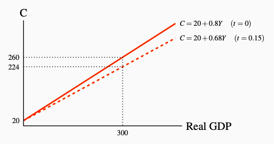
Figure 7.1: Net Taxes and Consumption
The net tax rate reduces disposable income relative to national income. The
marginal propensity to consume relative to national income falls, lowering
the slow of the C function from 0.8 to 0.68.

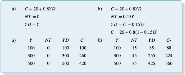
Example Box 7.1: A Numerical Example

In the absence of taxation, in example (a), national income Y and disposable income YD are the same. The consumption function C₁ shows how much households wish to consume at each level of national income, based on the numerical example.

With a proportional net tax rate of 0.15, households still consume $0.80 of each dollar of disposable income. Since as example (b) shows YD is now only 0.85 of Y, households consume only \(0.8 × 0.85 = 0.68\) of each extra dollar of national income, the effect of net taxes is to rotate the consumption function from C₁ to C₂ as in Figure 7.1. The slope of the consumption function is reduced.

A comparison of the numbers in examples (a) and (b) shows the effect of the tax rate at each income level. These numerical effects are also shown in the Figure 7.1.

Clearly, spending $0.68 of each extra dollar of national income implies a flatter consumption function, when plotted against national income, than spending $0.80 of each extra dollar of national income. The marginal tax rate t lowers disposable income at every level of national income and as a result lowers induced consumption expenditure. In a diagram the net tax rate lowers the slope of the expenditure function.

Aggregate expenditure and equilibrium output do not depend on whether the leakage is through saving (as when the MPC is low) or through imports or through taxes (as when the MPC multiplied by \((1−t)\) is low). Either way, the leakage prevents income from being recycled as expenditure on the output of producers.

If MPC is the marginal propensity to consume out of disposable income, and there is a proportional tax rate t, then the slope of the consumption function, the marginal propensity to consume out of national income, is given by:

\[\displaystyle\frac{\Delta{C}}{\Delta{Y}} = MPC \times (1 - t) = c(1 - t)\]

Government taxes and expenditure affect equilibrium national income and output and the position of the AD curve. To show this we start with an example in which investment expenditure is I₀, exports are X₀, imports are IM₀ + mY and the consumption function in terms of disposable income is \(C = C_0 + cYD\).

With the addition of government expenditure and taxes, aggregate expenditure equilibrium real GDP still determines equilibrium real GDP. The aggregate expenditure equation is:

\(\text{AE} = C + I + G + X - IM\)

Equilibrium real GDP is:

\[Y = C + I + G + X - IM\]

Then \(Y = C_0 + c(1 - t)Y + I_0 + G_0 + X_0 - IM_0 - mY\), and

\(Y = \displaystyle\frac {C_0 + I_0 + G_0 + X_0 - IM_0}{1 - c(1 - t) + m}\)

As before, equilibrium real GDP equals autonomous aggregate expenditure multiplied by the multiplier. With government added there is a new autonomous expenditure component G₀ and a new factor \((1 − t)\) in the multiplier, which lowers the slope of the AE function and the size of the multiplier. Table 7.3 illustrates.

The Effects of Both Government Expenditure and Taxation

Suppose the economy begins with no government and equilibrium output of 200. Assume autonomous consumption, investment and exports minus imports combined are \((20 + 20 + 50 − 10) = 80\). With a marginal propensity to consume out of disposable income of 0.80 and marginal propensity to import of 0.20, aggregate expenditure is \((80 × \text{multiplier}) = 80/[1 − (0.8 − 0.2)] = 80 × 2.5 = 200\), which is equal to output. Panel a) of Table 7.3 shows this equilibrium.

Table 7.3: The Effects of Net Taxes on Equilibrium GDP
a) This panel begins the illustration with an economy that does not have a
government sector. Autonomous expenditure of 80 and the multiplier of 2.5
gives equilibrium income Y_e = 200.
b) This panel adds a government sector that imposes a net tax rate of 12.5%
giving t = 0.125. Autonomous expenditure is still 80 but the net tax rate
lowers the slope of AE from 0.6 to 0.5, lowers the multiplier from 2.5 to
2.0. The new equilibrium income is Y'_e = 160.

Raising the net tax rate reduces equilibrium output because it reduces consumption expenditure, lowers the slope of the AE function and reduces the size of the multiplier. You will recall from Chapter 6 that the multiplier comes from the induced expenditure that is driven by autonomous expenditure. In the absence of net taxes, disposable income and national income are the same. Then the MPC is the change in consumption caused by a change in national income, slope of the AE function is \(MPC − MPM = c − m\), and the multiplier is \(1/(1−(c−m)) = 1/(1 − \text{slope of AE})\). A net tax rate \(t > 0\), or a change, \(\Delta{t} > 0\), reduces disposable income relative to national income, lowers the slope of the consumption function to \(c(1 − t) − m\), lowers the slope of AE, lowers the multiplier, lowers equilibrium output, and lowers aggregate demand. A cut in t, \(\Delta{t} < 0\), has the opposite effect.

Now introduce new autonomous expenditure \(G = 25\) from the government, taking total autonomous expenditure to 105. Also introduce a net tax rate \(t = 0.125\). The marginal propensity to consume out of national income (MPC) falls from 0.8 to 0.7, (0.8 × (1 − 0.125)), and the multiplier falls from 2.5 to \(1/(1 − (0.70 − 0.20) = 1/0.5 = 2.0\). Multiplying autonomous expenditure of 105 by 2.0 gives equilibrium output of 210, higher than the original equilibrium output of 200. Panel b) in Table 7.4 and Panel b) of Figure 7.2 illustrate this result.

Table 7.4: The Effects of Government Expenditure & Taxes on Equilibrium GDP
a) This panel begins with equilibrium in an economy without taxes of gov-
ernment expenditure. Autonomous expenditure is 80, the multiplier is 2.5
and equilibrium GDP is Y = 200.
b) This panel introduces government expenditure of G = 25 and net tax rev-
enue NT = 0.125Y. Government expenditure increases autonomous expen-
diture to 105 while net taxes reduce induced expenditure and the multiplier
to 2.0. Equilibrium GDP is Y = 210. This combination of increased gov-
ernment expenditure and taxes has a small positive effect on equilibrium.

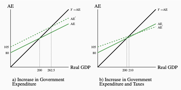
Figure 7.2: Government Expenditure, Taxes, and Equilibrium Real GDP
a) An increase in G of 25 with a multiplier of 2.5 increases equilibrium
GDP by 62.5.
b) An increase in G of 25 and a tax rate of g = 0.125 increase equilibrium
GDP by 10. The tax rate reduced the multiplier from 2.5 to 2.0.

The Multiplier Revisited

The multiplier relates changes in equilibrium national income to the changes in autonomous expenditures that cause them. The formula in Chapter 6 still applies.

\(\text{The multiplier} = \displaystyle\frac {1}{1 - \text{slope of AE}}\)

Without government and taxes, disposable income and national income are the same and when the marginal propensity to import is included and the multiplier is:

\(\displaystyle\frac{\Delta{Y}}{\Delta{A}} = \displaystyle\frac {1}{1 - MPC + MPM} = \displaystyle\frac {1}{1 - c + m}\)

With government and taxes proportional to income, the slope of the AE function is reduced.

\(\displaystyle\frac{\Delta{AE}}{\Delta{Y}} = c(1 - t) - m\)

The multiplier is smaller as a result, namely:

\(\displaystyle\frac {\Delta{Y}}{\Delta{A}} = \displaystyle\frac {1}{1 - c(1 - t) + m}\)

Table 7.4 provides numerical examples of these multipliers.

Now that we have seen that government expenditure and net tax taxes have effects on aggregate expenditure and equilibrium income, it is time to examine the effects of government budgets on AE, AD, and real GDP. The government implements fiscal policy through its budget.