
5.4: Oligopoly, Collusion, and Game Theory
- Last updated
- Save as PDF
- Page ID
- 43178

Collusion and Game Theory
Collusion occurs when oligopoly firms make joint decisions, and act as if they were a single firm. Collusion requires an agreement, either explicit or implicit, between cooperating firms to restrict output and achieve the monopoly price. This causes the firms to be interdependent, as the profit levels of each firm depend on the firm’s own decisions and the decisions of all other firms in the industry. This strategic interdependence is the foundation of game theory.
Game Theory = A framework to study strategic interactions between players, firms, or nations.
A game is defined as:
Game = A situation in which firms make strategic decisions that take into account each others’ actions and responses.
A game can be represented as a payoff matrix, which shows the payoffs for each possibility of the game, as will be shown below. A game has players who select strategies that lead to different outcomes, or payoffs. A Prisoner’s Dilemma is a famous game theory example where two prisoners must decide separately whether to confess or not confess to a crime. This is shown in Figure \(\PageIndex{1}\).
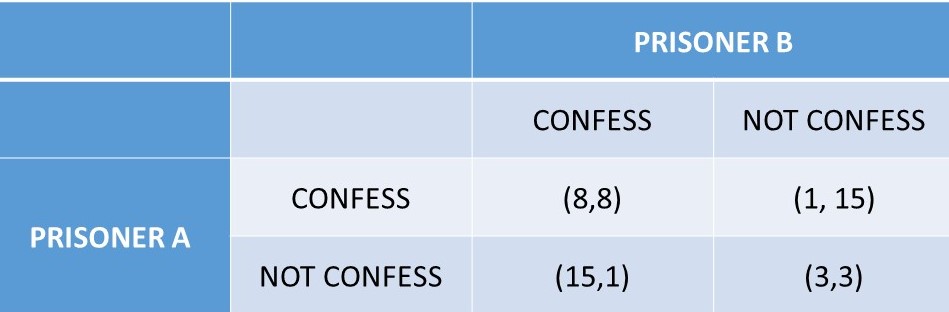
The police have some evidence that the two prisoners committed a crime, but not enough evidence to convict for a long jail sentence. The police seek a confession from each prisoner independently to convict the other accomplice. The outcomes, or payoffs, of this game are shown as years of jail sentences in the format \((A, B)\) where \(A\) is the number of years Prisoner \(A\) is sentenced to jail, and \(B\) is the number of years Prisoner \(B\) is sentenced to jail. The intuition of the game is that if the two Prisoners “collude” and jointly decide to not confess, they will both receive a shorter jail sentence of three years.
However, if either prisoner decides to confess, the confessing prisoner would receive only a single year sentence for cooperating, and the partner in crime (who did not confess) would receive a long 15-year sentence. If both prisoners confess, each receives a sentence of 8 years. This story forms the plot line of a large number of television shows and movies. The situation described by the prisoner’s dilemma is also common in many social and business interactions, as will be explored in the next chapter.
The outcome of this situation is uncertain. If both prisoners are able to strike a deal, and “collude,” or act cooperatively, they both choose to NOT CONFESS, and they each receive three year sentences, in the lower right hand outcome of Figure \(\PageIndex{1}\). This is the cooperative agreement: \((\text{NOT, NOT}) = (3,3)\). However, once the prisoners are in this outcome, they have a temptation to “cheat” on the agreement by choosing to CONFESS, and reducing their own sentence to a single year at the expense of their partner. How should a prisoner proceed? One way is to work through all of the possible outcomes, given what the other prisoner chooses.
A Solution to the Prisoner’s Dilemma: Dominant Strategy
(1) If \(\text{B CONF, A}\) should \(\text{CONF } (8 < 15)\)
(2) If \(\text{B NOT, A}\) should \(\text{CONF } (1 < 3)\)
…\(A\) has the same strategy no matter what \(B\) does: \(\text{CONF}\).
(3) If \(\text{A CONF, B}\) should \(\text{CONF } (8 < 15)\)
(4) If \(\text{A NOT, B}\) should \(\text{CONF } (1 < 3)\)
…\(B\) has the same strategy no matter what \(A\) does: \(\text{CONF}\).
Thus, \(A\) chooses to \(\text{CONFESS}\) no matter what. This is called a Dominant Strategy, since it is the best choice given any of the strategies selected by the other player. Similarly, \(\text{CONFESS}\) is the dominant strategy for prisoner \(B\).
Dominant Strategy = A strategy that results in the highest payoff to a player regardless of the opponent’s action.
The Equilibrium in Dominant Strategies for the Prisoner’s Dilemma is \((\text{CONF, CONF})\). This is an interesting outcome, since each prisoner receives eight-year sentences: \((8, 8)\). If they could only cooperate, they could both be better off with much lighter sentences of three years.
A second example of a game is the decision of whether to produce natural beef or not. Natural beef is typically defined as beef produced without antibiotics or growth hormones. The definition is difficult, since it means different things to different people, and there is no common legal definition. This game is shown in Figure \(\PageIndex{2}\), where Cargill and Tyson decide whether to produce natural beef.
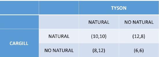
There are two players in the game: Cargill and Tyson. Each firm has two possible strategies: produce natural beef or not. The payoffs in the payoff matrix are profits (million USD) for the two companies: \((π_{Cargill}, π_{Tyson})\).
Strategy = Each player’s plan of action for playing a game.
Outcome = A combination of strategies for players.
Payoff = The value associated with possible outcomes.
In this game, profits are made from the premium associated with natural beef. If only one firm produced natural beef,
Dominant Strategy for the Natural Beef Game
(1) If \(\text{TYSON NAT, CARGILL}\) should \(\text{NAT } (10 > 8)\)
(2) If \(\text{TYSON NO, CARGILL}\) should \(\text{NAT } (12 > 6)\)
…\(\text{CARGILL}\) has the same strategy no matter what \(\text{TYSON}\) does: \(\text{NAT}\).
(3) If \(\text{CARGILL NAT, TYSON}\) should \(\text{NAT } (10 > 8)\)
(4) If \(\text{CARGILL NO, TYSON}\) should \text{NAT} (12 > 6)\)
…\(\text{TYSON}\) has the same strategy no matter what \(\text{CARGILL}\) does: \(\text{NAT}\).
Both firms choose to produce natural beef, no matter what, so this is a Dominant Strategy for both firms. The Equilibrium in Dominant Strategies is \((\text{NAT, NAT})\). The outcome of this game demonstrates why all beef processors have moved quickly into the production of natural beef in the past few years, and are all earning higher levels of profits. Beef producers have also moved rapidly into organic beef, local beef, grass-fed beef, and even plant-based “beef.”
Prisoner’s Dilemmas are very common in oligopoly markets: gas stations, grocery stores, garbage companies are frequently in this situation. If all oligopolists in a market could agree to raise the price, they could all earn higher profits. Collusion, or the cooperative outcome, could result in monopoly profits. In the USA, explicit collusion is illegal. “Price setting” is outlawed to protect consumers. However, implicit collusion (tacit collusion) could result in monopoly profits for firms in a prisoner’s dilemma. For example, if gas stations in a city such as Manhattan, Kansas all matched a higher price, they could all make more money. However, there is an incentive to cheat on this implicit agreement by cutting the price and attracting more customers away from the other firms to your own gas station. Firms in a cooperative agreement are always tempted to break the agreement to do better.
The Nash Equilibrium calculated for the three oligopoly models (Cournot, Bertand, and Stackelberg) is a noncooperative equilibrium, as the firms are rivals and do not collude. In these models, firms maximize profits given the actions of their rivals. This is common, since collusion is illegal and price wars are costly. How do real-world oligopolists deal with prisoner’s dilemmas is the topic of the next section.
Rigid Prices: Kinked Demand Curve Model
Oligopolists have a strong desire for price stability. Firms in oligopolies are reluctant to change prices, for fear of a price war. If a single firm lowers its price, it could lead to the Bertrand equilibrium, where price is equal to marginal costs, and economic profits are equal to zero. The kinked demand curve model was developed to explain price rigidity, or oligopolist’s desire to maintain price at the prevailing price, \(P^*\).
The kinked demand model asserts that a firm will have an asymmetric reaction to price changes. Rival firms in the industry will react differently to a price change, which results in different elasticities for price increases and price decreases.
(1) If a firm increases price, \(P > P^*\), other firms will not follow
… the firm will lose most customers, the demand is highly elastic above \(P^*\)
(2) If a firm decreases price, \(P < P^*\), other firms will follow immediately
…each firm will keep the same customers, demand is inelastic below \(P^*\)
The kinked demand curve is shown in Figure \(\PageIndex{3}\), where the different reactions of other firms leads to a kink in the demand curve at the prevailing price \(P^*\).
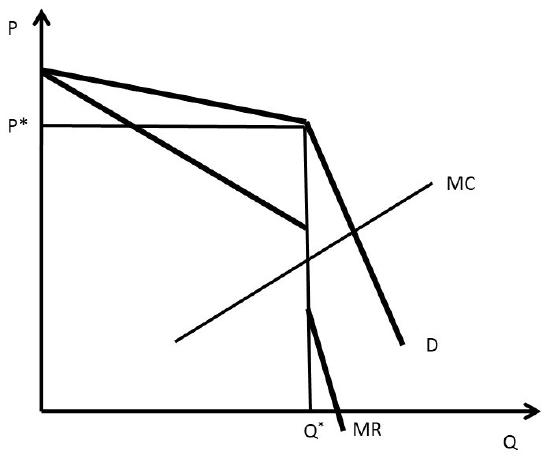
In the kinked demand curve model, \(MR\) is discontinuous, due to the asymmetric nature of the demand curve. For linear demand curves, \(MR\) has the same y-intercept and two times the slope… resulting in two different sections for the \(MR\) curve when demand has a kink. The graph shows how price rigidity occurs: any changes in marginal cost result in the same price and quantity in the kinked demand curve model. As long as the \(MC\) curve stays between the two sections of the \(MR\) curve, the optimal price and quantity will remain the same.
One important feature of the kinked demand model is that the model describes price rigidity, but does not explain it with a formal, profit-maximizing model. The explanation for price rigidity is rooted in the prisoner’s dilemma and the avoidance of a price war, which are not part of the kinked demand curve model. The kinked demand model is criticized because it is not based on profit-maximizing foundations, as the other oligopoly models.
Two additional models of pricing are price signaling and price leadership.
Price Signaling = A form of implicit collusion in which a firm announces a price increase in the hope that other firms will follow suit.
Price signaling is common for gas stations and grocery stores, where price are posted publically.
Price Leadership = A form of pricing where one firm, the leader, regularly announces price changes that other firms, the followers, then match.
There are many examples of price leadership, including General Motors in the automobile industry, local banks may follow a leading bank’s interest rates, and US Steel in the steel industry.
Dominant Firm Model: Price Leadership
A dominant firm is defined as a firm with a large share of total sales that sets a price to maximize profits, taking into account the supply response of smaller firms. The dominant firm model is also known as the price leadership model. The smaller firms are referred to as the “fringe.” Let \(F =\) fringe, or many relatively small competing firms in the same industry as the dominant firm. Let \(Dom =\) the dominant firm. The market demand for the good \((D_{mkt})\) is equal to the sum of the demand facing the dominant firm \((D_{dom})\) and the demand facing the fringe firms \((D_F)\).
\[D_{dom} = D_{mkt} – D_F \nonumber\]
Total quantity (QT) is also the sum of output produced by the dominant and fringe firms.
\[Q_T = Q_{dom} + Q_F \nonumber\]
The dominant firm model is shown in Figure \(\PageIndex{4}\). The supply curve for the fringe firms is given by \(S_F\), and the marginal cost of the dominant firm is \(MC_{dom}\). Recall that the marginal cost curve is the firm’s supply curve. The dominant firm has the advantage of lower costs due to economies of scale. In what follows, the dominant firm will set a price, allow the fringe firms to produce as much as they desire, and then find the profit-maximizing quantity and price with the remainder of the market.
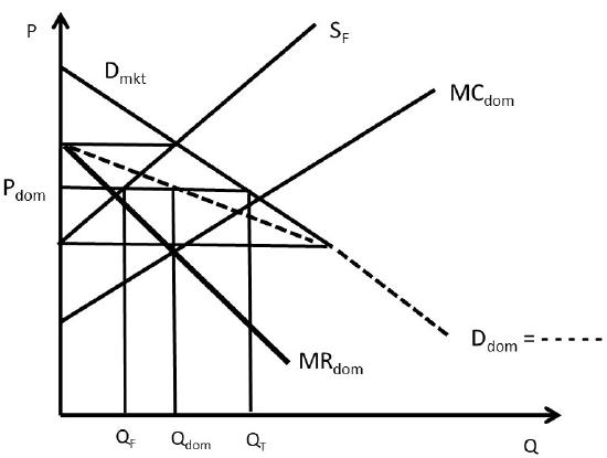
To find the profit-maximizing level of output, the dominant firm first finds the demand curve facing the dominant firm (the dashed line in Figure \(\PageIndex{4}\)), then sets marginal revenue equal to marginal cost. The dominant firm’s demand curve is found by subtracting the supply of the fringe firms \((S_F)\) from the total market demand \((D_{mkt})\).
\[D_{dom} = D_{mkt} – S_F \nonumber\]
The dominant firm demand curve is found by the following procedure. The y-intercept of the dominant firm’s demand curve occurs where \(S_F\) is equal to the \(D_{mkt}\). At this point, the fringe firms supply the entire market, so the residual facing the dominant firm is equal to zero. Therefore, the demand curve of the dominant firm starts at the price where fringe supply equals market demand. The second point on the dominant firm demand curve is found at the y-intercept of the fringe supply curve \((S_F)\). At any price equal to or below this point, the supply of the fringe firms is equal to zero, since the supply curve represents the cost of production. At this point, and all prices below this point, the market demand \((D_{mkt})\) is equal to the dominant firm demand \((D_{dom})\). Thus, the dashed line below the y-intercept of the fringe supply is equal to the market demand curve. The dominant firm demand curve for prices above this point is found by drawing a line from the y-intercept at price \((S_F = D_{mkt})\) to the point on the market demand curve at the price of the \(S_F\) y-intercept. This is the dashed line above the \(S_F\) y-intercept.
Once the dominant firm demand curve is identified, the dominant firm maximizes profits by setting marginal revenue equal to marginal cost at quantity \(Q_{dom}\). This level of output is then substituted into the dominant firm demand curve to find the price \(P_{dom}\). The fringe firms take this price as given, and produce \(Q_F\). The sum of \(Q_{dom}\) and \(Q_F\) is the total output \(Q_T\).
In this way, the dominant firm takes into account the reaction of the fringe firms while making the output decision. This is a Nash equilibrium for the dominant firm, since it is taking the other firms’ behavior into account while making its strategic decision. The model effectively captures an industry with one dominant firm and many smaller firms.
Cartels
A cartel is a group of firms that have an explicit agreement to reduce output in order to increase the price.
Cartel = An explicit agreement among members to reduce output to increase the price.
Cartels are illegal in the United States, as the cartel is a form of collusion. The success of the cartel depends upon two things: (1) how well the firms cooperate, and (2) the potential for monopoly power (inelastic demand).
Cooperation among cartel members is limited by the temptation to cheat on the agreement. The Organization of Petroleum Exporting Countries (OPEC) is an international cartel that restricts oil production to maintain high oil prices. This cartel is legal, since it is an international agreement, outside of the American legal system. The oil cartel’s success depends on how well each member nation adheres to the agreement. Frequently, one or more member nations increases oil production above the agreement, putting downward pressure on oil prices. The cartel’s success is limited by the temptation to cheat. This cartel characteristic is that of a prisoner’s dilemma, and collusion can be best understood in this way.
A collusive agreement, or cartel, results in a circular flow of incentives and behavior. When firms in the same industry act independently, they each have an incentive to collude, or cooperate, to achieve higher levels of profits. If the firms can jointly set the monopoly output, they can share monopoly profit levels. When firms act together, there is a strong incentive to cheat on the agreement, to make higher individual firm profits at the expense of the other members. The business world is competitive, and as a result oligopolistic firms will strive to hold collusive agreements together, when possible. This type of strategic decisions can be usefully understood with game theory, the subject of the next two Chapters.