5.3: Lancaster’s (1966) Characteristics Model

Last updated
Save as PDF

Page ID: 45361

$ \newcommand{\vecs}[1]{\overset { \scriptstyle \rightharpoonup} {\mathbf{#1}} } $ $ \newcommand{\vecd}[1]{\overset{-\!-\!\rightharpoonup}{\vphantom{a}\smash {#1}}} $$\newcommand{\id}{\mathrm{id}}$ $ \newcommand{\Span}{\mathrm{span}}$ $ \newcommand{\kernel}{\mathrm{null}\,}$ $ \newcommand{\range}{\mathrm{range}\,}$ $ \newcommand{\RealPart}{\mathrm{Re}}$ $ \newcommand{\ImaginaryPart}{\mathrm{Im}}$ $ \newcommand{\Argument}{\mathrm{Arg}}$ $ \newcommand{\norm}[1]{\| #1 \|}$ $ \newcommand{\inner}[2]{\langle #1, #2 \rangle}$ $ \newcommand{\Span}{\mathrm{span}}$ $\newcommand{\id}{\mathrm{id}}$ $ \newcommand{\Span}{\mathrm{span}}$ $ \newcommand{\kernel}{\mathrm{null}\,}$ $ \newcommand{\range}{\mathrm{range}\,}$ $ \newcommand{\RealPart}{\mathrm{Re}}$ $ \newcommand{\ImaginaryPart}{\mathrm{Im}}$ $ \newcommand{\Argument}{\mathrm{Arg}}$ $ \newcommand{\norm}[1]{\| #1 \|}$ $ \newcommand{\inner}[2]{\langle #1, #2 \rangle}$ $ \newcommand{\Span}{\mathrm{span}}$$\newcommand{\AA}{\unicode[.8,0]{x212B}}$

In the neoclassical model of consumer choice described above, the consumer has preferences that can be represented by a utility function. The solution to the consumer’s choice involves a constrained optimization problem wherein the consumer seeks the bundle that returns the highest utility possible given his or her budget set. The benefit of the neoclassical model is that it provides a framework for examining the role of price changes, income changes, and (in some cases) preference changes on consumer behavior. You saw in Demonstration 5.2.2, for example, that given some reasonable assumptions, the solution to the neoclassical choice model results in demand functions that are downward sloping in own-price and that could depend on prices of related substitute and complement goods as well as consumer income.

An alternative formulation of the consumer’s choice problem is provided by Lancaster (1966). This model is similar to the neoclassical model in that it relies on the same basic premise: Consumers seek the best bundle of goods given an affordability constraint. However, it differs from the neoclassical model in terms of how preferences and budget sets are formulated.

Preferences in the Lancaster Model

The essential difference in the Lancaster model is that the consumer views a purchased good as a bundle of characteristics. For example, the consumer is not interested in a half gallon of orange juice per se. Rather he or she is interested in characteristics such as vitamin C, potassium, a sweet and tart taste sensation, carbohydrates for energy, dietary fiber, etc. The consumer could satisfy the desire for these characteristics through orange juice or through several other products. For example, grapefruit juice might provide similar micro-nutrient characteristics to orange juice but would differ in terms of the taste characteristics provided (less sweet with a slightly bitter aftertaste) and macro-nutrients (perhaps slightly fewer calories). Concord grape juice would lack the tartness of orange juice, provide a taste sensation that is more sweet, would likely contain more calories, provide more or less of certain micro-nutrients, and would provide a mouth-feel different from either orange juice or grapefruit juice. The point to be made here is that orange juice, grapefruit juice, and Concord grape juice are more than just products, they are delivery mechanisms for a variety of characteristics that the consumer may value.

Utility in the Lancaster Model

In Lancaster’s model, the consumer has preferences that can be represented by a utility function. However, preferences and utility levels are defined in terms of characteristics of purchased goods and services. A utility function in Lancaster’s framework can be defined as follows:

$U = f(c_{11}, c_{12}, c_{13}, \cdots, c_{1N}, c_{21}, c_{22}, c_{23}, \cdots, c_{2N}, \cdots, c_{M1}, c_{M2}, C_{M3}, \cdots, c_{MN}),$

where $c_{ij}$ is the amount of the $i^{th}$ characteristic contained in one unit of the $j^{th}$ purchased good, $i = 1, 2, 3, \cdots, M$ and $j = 1, 2, 3, \cdots, N.$

For example, it would be possible to identify and measure characteristics in three juice products: orange juice ($Q_{1}$) , grapefruit juice ($Q_{2}$), and Concord grape juice ($Q_{3}$). Suppose, for simplicity, that consumers care only about two characteristics: sweetness (characteristic 1) and tartness (characteristic 2). In this case, the $c_{ij}$ terms in the consumer’s utility function would be interpreted as follows:

$c_{11}$ = the amount of characteristic 1 (sweetness) in product 1 (orange juice)
$c_{12}$= the amount to characteristic 1 (sweetness) in product 2 (grapefruit juice)
$c_{13}$ = the amount of characteristic 1 (sweetness) in product 3 (Concord grape juice)
$c_{21}$ = the amount of characteristic 2 (tartness) in product 1 (orange juice)
$c_{22}$= the amount characteristic 2 (tartness) in product 2 (grapefruit juice)
$c_{23}$= the amount of characteristic 2 (tartness) in product 3 (Concord grape juice)

The formulation of preferences in the Lancaster model clearly has implications for product design and marketing. Within one single product, there can be the opportunity to adjust characteristics being offered to consumers with different tastes. For example, consider ready-to-serve orange juice in the typical supermarket. You will see variations in terms of pulp, whether the product is from concentrate, and whether the product has been fortified with other nutrients not naturally found in orange juice (e.g., calcium). Basically, food marketers understand that altering the characteristics of a product can make it more attractive to certain consumer segments.

The Lancaster model does assume that the characteristics that are of interest to consumers can be measured. In many cases, this would be straightforward. For example, consider an automobile. Characteristics that might be important to the consumer include horsepower, fuel efficiency, head room, leg room, number of doors, whether the vehicle is four-wheel drive, and so forth. Some characteristics that are important to the consumer such as reliability and smoothness of ride might be more difficult to measure. However, there are third-party entities that provide ratings for experience characteristics like reliability and handling. Moreover, the consumer will generally test drive the vehicle to assess some of these characteristics before purchase. In the case of food products, sensory labs with specialized equipment and trained sensory panelists can provide quantitative measures of characteristics such as texture, firmness, mouth-feel, aftertastes, and other attributes of the product.

Budget Sets in the Lancaster Model

Provided that characteristics can be measured, it is possible to construct a budget constraint for the Lancaster model. Remember that in the Lancaster model, consumers care about characteristics. Purchased goods matter to the consumer only because of the characteristics contained therein. In other words, utility is derived indirectly from purchased goods and services. This being the case, the budget constraint for Lancaster’s model needs to reflect the amount of characteristics the consumer can afford.

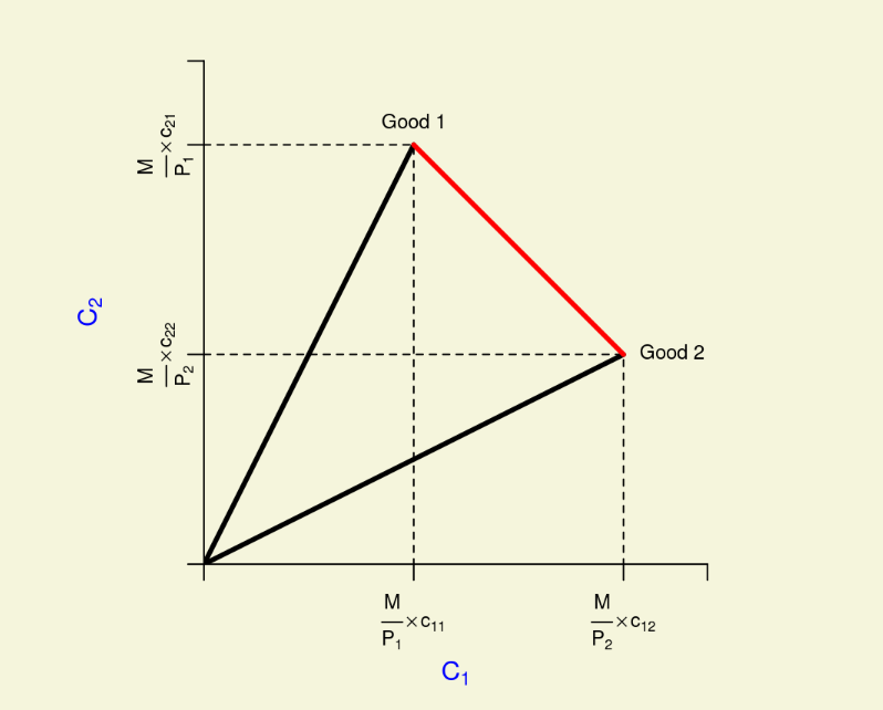
Figure $\PageIndex{1}$ provides a diagram of a Lancaster-type budget set for two characteristics. Following the earlier conventions, let $P_{1}$ and $P_{2}$ be the prices of products 1 and 2, respectively, and let M be the consumer’s budget. Notice that in Figure $\PageIndex{1}$, the characteristics are on the vertical and horizontal axis. The consumer cannot buy characteristics directly, but obtains characteristics by purchasing products 1 and 2. Thus, the affordable amounts of products 1 and 2 need to be converted into the characteristics they deliver. In Figure $\PageIndex{1}$, each purchased good is a vector extending from the origin. The affordable set of characteristics in Figure $\PageIndex{1}$ is contained within the triangular shaped area inside the two product vectors and the red line segment connecting the endpoints of the two vectors. The consumer can obtain any point inside this triangle by buying goods 1 and 2 in the appropriate combination. The efficient consumption frontier (in red) consists of combinations of products that provide the most characteristics for the consumer’s dollar. This efficient consumption frontier is analogous to the budget frontier in the neoclassical model.

Figure $\PageIndex{1}$: **The efficient consumption fronteir (in red) for two characteristics, $C_{1}$ and $C_{2}$.**

Choice in the Lancaster Model

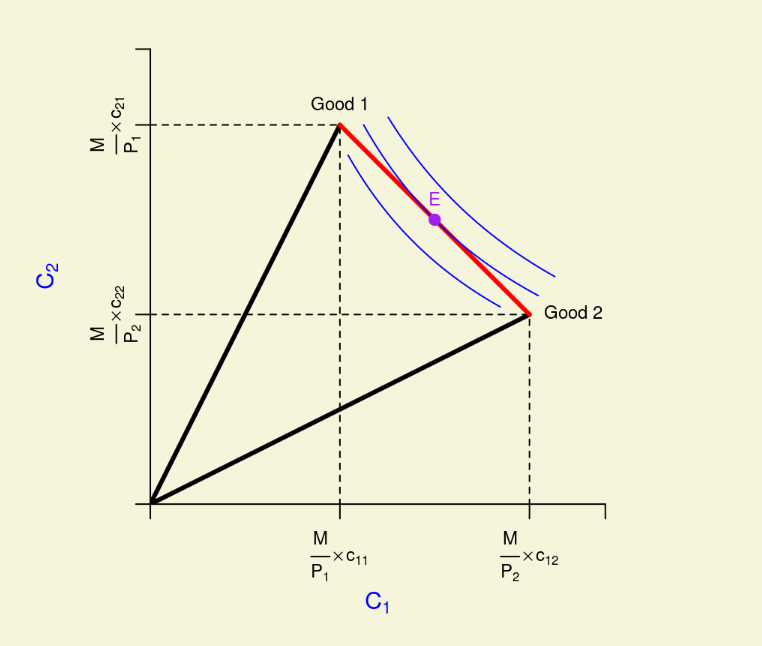
In the Lancaster Model, the consumer’s optimal choice is the bundle of goods that provides the combination of characteristics that provide him or her with the highest level of utility given the affordability constraint. If the consumer has monotonic preferences over the two preferences, this choice will occur somewhere on the efficient consumption frontier. In Figure $\PageIndex{2}$, a consumer’s indifference curves are imposed over the affordable set, and the optimal choice occurs at point E. In this particular example, the consumer spends half of his or her budget on good 1 and half on good 2. This happens to occur at a tangency between the line segment constituting the efficient consumption frontier and the consumer’s indifference curve. However, optimal choices need not be points of tangency in the Lancaster model even if preferences are monotonic and convex over the characteristics. Had these preferences been drawn differently, the optimal choice could have occurred at one of the product vector endpoints. You will see this in the example that follows.

An Example

Consider the fictional characteristic and price data for red delicious (RD) and golden delicious (GD) apples as presented in Table $\PageIndex{1}$. As should be clear from the table, RD apples are sweeter than GD apples but GD apples are crispier than RD apples in this example. Consider a consumer who purchases apples because he or she values the attributes of sweetness and crispiness.

Table $\PageIndex{1}$. Fictional Characteristic and Price Data for the Apple Example

Characteristic	Red Delicious (RD) Apple	Golden Delicious (GD) Apple
Crispiness	1 unit	2 units
Sweetness	2 units	1 unit

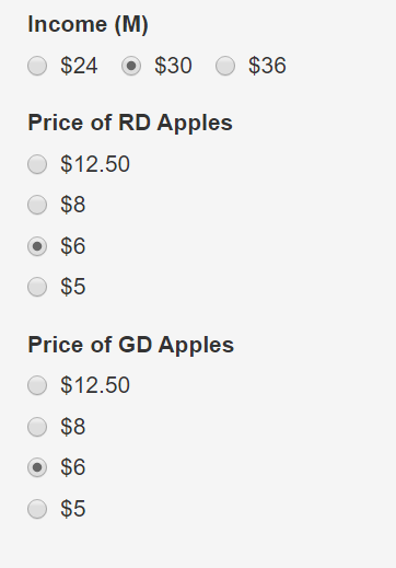
The information in Table $\PageIndex{1}$ is reflected below in Demonstration $\PageIndex{1}$. As shown in the demonstration, the price of each type of apple is initially $6 per unit and the consumer has an initial budget of $30 that is used to purchase apples ($M = $30$). If the consumer spends all of the $30 budget on RD apples, he or she could obtain five RD apples in total. Multiplying this total by the value of the characteristics per apple indicates that these five RD apples would provide a total of five units of crispiness and 10 units of sweetness. Similarly, if the consumer spends all the budget on GD apples, he or she could obtain five GD apples in total, which would provide 10 units of crispiness and five units of sweetness. This sets up the initial values in the demonstration.

Demonstration $\PageIndex{1}$. Efficient Consumption Frontier for Example of RD and GD Apples

Use Demonstration $\PageIndex{1}$ to adjust the income and the price of the apples. Make note of the following features from the demonstration:

The efficient consumption frontier can collapse to a point if one of the products becomes noncompetitive. To see this, change the RD price to $5 and set the GD price to $12.50. In this case, a consumer that cared only about crispiness could still get more crispiness by buying RD apples. RD apples dominate GD apples in terms of both crispiness and sweetness meaning that GD is priced out of the market. Similarly, if you set the RD price to $12.50 and the GD price to $5, the efficient consumption frontier collapses to a point that includes only GD apples. GD apples become the most efficient mechanism by which to obtain both sweetness and crispiness and RD is priced out of the market.
An increase in price causes the product vector to contract radially towards the origin.
A decrease in price causes the product vector to expand radially away from the origin.
A change in income causes both vectors to contract or expand proportionately. The efficient consumption frontier shifts in the same direction of the income change. If both products are competitive, the new efficient consumption frontier is parallel to the old.

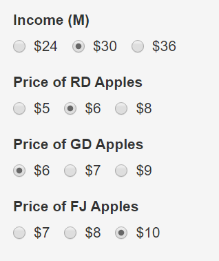
Now let us complicate the example by assuming that Fuji apples have all the sweetness of a RD apple and all the crispiness of a GD apple. The characteristics of the Fuji apple are presented in Table $\PageIndex{2}$ below. This is clearly a better apple, but let us assume that it is also more costly to grow. In Demonstration $\PageIndex{2}$, the Fuji apple is priced initially at $10. Notice that at $10, the Fuji apple is not on the efficient consumption frontier. Even though it is a better apple in terms of its attributes, it is too costly and is not market feasible at $10. Consumers can obtain more of the characteristics in question by purchasing RD apples, GD apples, or some combination thereof.

Table $\PageIndex{2}$. Updated Characteristics Table for the Apple Example
Characteristic	Red Delicious (RD) Apple	Golden Delicious (GD) Apple	Fuji (FJ) Apple
Crispiness	1 unit	2 units	2 units
Sweetness	2 units	1 unit	2 units

Demonstration $\PageIndex{2}$. The Expanded Example

If the price of the Fuji apples is reduced to $8 in Demonstration $\PageIndex{2}$, it becomes competitive with the other two apples. At an even lower price of $7, Fuji apples start to push out the efficient frontier, causing it to kink. In this case, the Fuji apple becomes the best choice for those consumers who like a balance of crispiness and sweetness. Note that RD and GD apples are still on the frontier when Fuji apples are priced at $7. This is because consumers who have strong preferences for sweetness but not crispiness or strong preferences for crispiness but not sweetness may still find it optimal to purchases bundles with RD or GD apples, respectively.

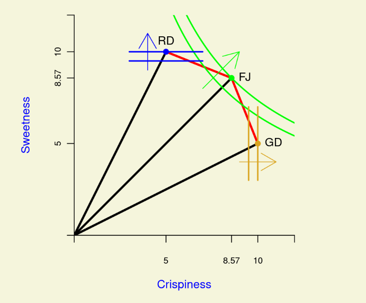
This is illustrated in Figure $\PageIndex{3}$ below. Figure $\PageIndex{3}$, shows indifference curves for three consumers. One consumer has the horizontal indifference curves shown in blue. This consumer cares only about sweetness and nothing about crispiness. His or her utility is maximized by purchasing all RD apples because this provides the largest amount of sweetness. Another consumer has the vertical indifference curves shown in yellow. This consumer cares only about crispiness and nothing about sweetness. He or she maximizes utility by purchasing only GD Apples. The consumer with the typically shaped and strictly convex indifference curves shown in green likes both crispiness and sweetness. He or she maximizes utility by purchasing the Fuji apples.

Figure $\PageIndex{3}$: Choice by consumers with different preferences shown in blue, green, and yellow. Characteristics reflected in the figure are from Table $\PageIndex{2}$. Other assumptions are $M = $30$, $PRD = $6$, $PGD = $6$, and $PFJ = $7$. Arrows point in the direction of increasing preferences.

Hedonic Pricing Models

In Lancaster’s framework, characteristics are the things that matter in the consumer’s utility function. The consumer gets characteristics by purchasing goods and services that contain them. When a market price is observed, the price is for a product that probably reflects a number of characteristics. You cannot observe the value of individual characteristics directly. Continuing the automobile example above, the price of the automobile reflects horsepower along with several other characteristics. You may observe that cars with higher horsepower also tend to have higher price tags. This suggests that it should be possible to construct a model to get an estimate of the implicit price for horsepower. Such a model is called a hedonic pricing model. A hedonic pricing model could be specified as follows:

$p = f(c_{1}, c_{2}, \cdots, c_{M}),$

where $p$ is price of the product in question and $c_{1}, c_{2}, \cdots, C_{M}$ are levels of different characteristics.

A hedonic pricing model can be used to obtain the implicit marginal value of a characteristic. For example, if $p$ is the price of an automobile and $c_{1}$ is horsepower, then $\dfrac{\Delta p}{\Delta c_{1}}$ (the slope coefficient for $c_{1}$) is the increase in automobile price that one would expect to result from increasing horsepower by a small amount.

As an example, suppose that you were asked to specify a hedonic pricing model for retail strip steaks. You might use something such as

$p = f(weight, \: thickness, \: color, \: quality, \: freshness)$

You could measure weight (g) and thickness (cm). There are techniques for quantifying color and quality could be measured in terms of internal marbling and/or through a series of binary (0 or 1) variables to control for USDA quality grade (prime, choice, select, and so forth). These grades take marbling into account. Freshness might be measured in terms of days remaining before the “sale by” date.

A hedonic pricing model provides information about the returns that could be expected by improvements to one or more of the characteristics. In the case of our retail strip steak, it may be possible to increase freshness by using vacuum packaging. Before investing in such a technology, it would be nice to know how much consumers would be willing to pay for this product improvement. Vacuum packaging could darken the color and result in a steak that is purplish rather than a bright red. It is possible that despite enhanced freshness, consumers would pay less for vacuum packed steaks because they view the darker color to be undesirable. A hedonic pricing model could be very useful decision tool in this type of a situation.