7.5: Profit Maximization in an Oligopoly

Last updated
Save as PDF

Page ID: 45377

$ \newcommand{\vecs}[1]{\overset { \scriptstyle \rightharpoonup} {\mathbf{#1}} } $ $ \newcommand{\vecd}[1]{\overset{-\!-\!\rightharpoonup}{\vphantom{a}\smash {#1}}} $$\newcommand{\id}{\mathrm{id}}$ $ \newcommand{\Span}{\mathrm{span}}$ $ \newcommand{\kernel}{\mathrm{null}\,}$ $ \newcommand{\range}{\mathrm{range}\,}$ $ \newcommand{\RealPart}{\mathrm{Re}}$ $ \newcommand{\ImaginaryPart}{\mathrm{Im}}$ $ \newcommand{\Argument}{\mathrm{Arg}}$ $ \newcommand{\norm}[1]{\| #1 \|}$ $ \newcommand{\inner}[2]{\langle #1, #2 \rangle}$ $ \newcommand{\Span}{\mathrm{span}}$ $\newcommand{\id}{\mathrm{id}}$ $ \newcommand{\Span}{\mathrm{span}}$ $ \newcommand{\kernel}{\mathrm{null}\,}$ $ \newcommand{\range}{\mathrm{range}\,}$ $ \newcommand{\RealPart}{\mathrm{Re}}$ $ \newcommand{\ImaginaryPart}{\mathrm{Im}}$ $ \newcommand{\Argument}{\mathrm{Arg}}$ $ \newcommand{\norm}[1]{\| #1 \|}$ $ \newcommand{\inner}[2]{\langle #1, #2 \rangle}$ $ \newcommand{\Span}{\mathrm{span}}$$\newcommand{\AA}{\unicode[.8,0]{x212B}}$

To introduce oligopoly, consider an example where there are only two firms that supply the market, Firm A and Firm B. This is the simplest form of oligopoly (a duopoly). To simplify the example further, assume that both firms have identical variable cost functions $VC= 20Q_{i}$, where $i \in [A, B]$. This means that the marginal cost facing each firm is $MC = 20$. Finally, suppose that the inverse demand curve for this industry is $P = 200 - 2Q_{A}-2Q_{B}$

Just to be clear, $Q_{A}$ is the amount that Firm A produces and $Q_{B}$ is the amount that Firm B produces.

Because the inverse demand curve is linear, it is easy to find marginal revenue. Note that Firm A can only choose $Q_{A}$. The amount of $Q_{B}$ is outside of Firm A’s control, so the $Q_{B}$ component of the industry inverse demand curve becomes part of the intercept of the inverse demand curve that Firm A actually faces. With this in mind, the MR for Firm A is

$MR_{A}=200-4Q_{A}-2Q_{B}$.

Set $MR=MC$ for Firm A to find profit maximizing quantity for Firm A conditional on Firm B’s output choice

$200-4Q_{A}-2Q_{B} = 200 \Rightarrow Q_{A} = 45 - \dfrac{1}{2} Q_{B}$.

This is known as the reaction function for Firm A. It indicates Firm A’s optimal quantity choice as a function of Firm B’s quantity. In other words, it says how Firm A’s quantity will react to a change in Firm B’s quantity.

Next, repeat the above steps to find profit maximizing quantity for Firm B conditional on Firm A’s output choice. MR for Firm B is

$MR_{B} = 200 - 2Q_{A} -4Q_{B}$.

Set MR = MC for Firm B and solve for $Q_{B}$ to get Firm B’s reaction function.

$200-2Q_{A} - 4Q_{B} = 20 \Rightarrow Q_{B} = 45 \dfrac{1}{2} Q_{A}$

Cournot Nash Equilibrium

A Cournot Nash equilibrium occurs where the reaction functions for these two firms intersect (see Figure $\PageIndex{1}$). To find the equilibrium, we can substitute Firm B’s reaction function into the reaction function for Firm A:

\(Q_{A} = 45 - \dfrac{1}{2}(45 - \dfrac{1}{2}Q_{A})

Now there is one equation and one unknown. Solving for $Q_{A}$ provides $Q_{A} = 30$. Putting this back into Firm B’s reaction function, we find that $Q_{B} = 30$ as well.

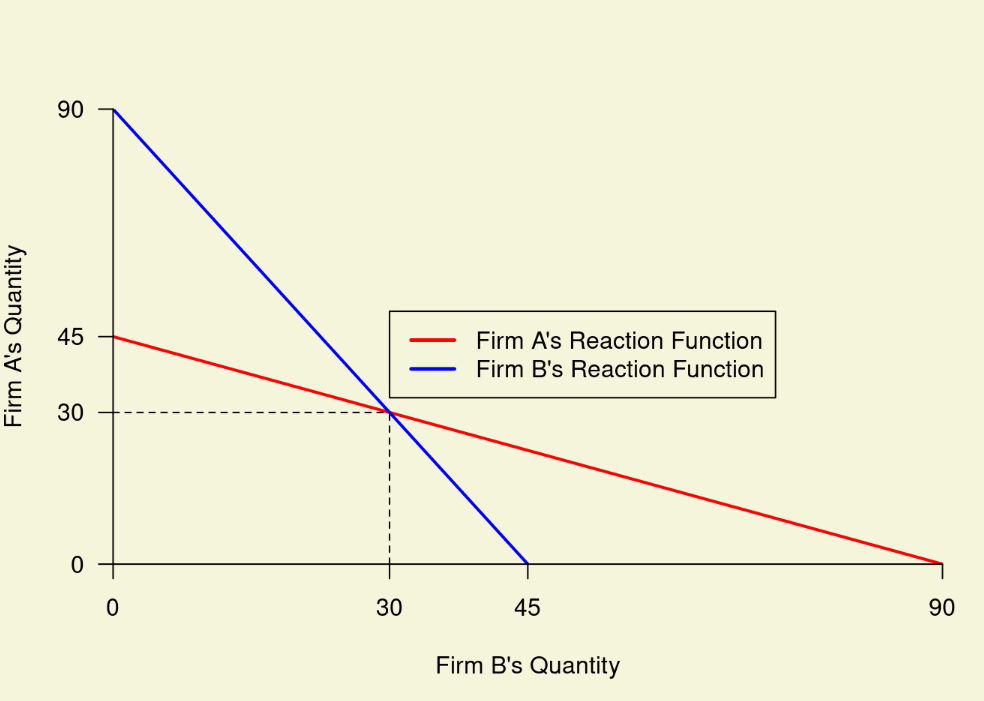
Figure $\PageIndex{1}$: **Cournot Nash Equilibrium for Two Firms in Oligopoly**

Finally, we can find the price at the Cournot Nash Equilibrium by putting these quantities into the industry inverse demand curve to get

$P = 200 - 2(30) - 2(30)= 80.$

A Nash equilibrium refers to a situation wherein each agent chooses a strategy that maximizes his or her payoffs conditional on the strategies of all other agents. In the example above, the strategy variable is the quantity to be placed on the market. The Cournot equilibrium is a Nash equilibrium because 30 units is the optimal quantity to be placed on the market by Firm A, given that Firm B places 30 units on the market and vice versa. This type of equilibrium, is named after John Forbes Nash, Jr., a mathematician who was awarded the Nobel Prize in Economics for this idea. The model in this example is one of Cournot oligopoly, wherein competition is on quantity. This model is named after another mathematician, Antoine Augustin Cournot.

The Prisoners’ Dilemma

The Cournot Nash equilibrium outcome is not optimal from the standpoint of the two oligopolists because there exists another feasible outcome that provides each firm with a higher level profits. To demonstrate, suppose that the two firms merged. Now there would be just one combined quantity to put on the market $Q_{M} = Q_{A} + Q_{B}$. The inverse demand equation for the combined firm would be

$P = 200 - 2Q_{M}.$

Assuming that the merger does not impact marginal cost, the marginal cost would still be $MC=20$, but marginal revenue for the merged firm would now be $P-200 -4Q_{M}$. Setting marginal revenue equal to marginal cost and solving for $Q_{M}$ results in the merged firm (now a monopolist) putting a quantity of 45 units on the market and charging a price of $P=200-2(45) = $110$. The point here is that technically it would be feasible for the oligopolists to each put half of this amount, 22.5 units, on the market. The industry price would be $110, and they would each be more profitable.

At the Cournot Nash equilibrium, each firm makes profits above fixed costs of $(80-20) \times 30 = $1800$.
By each putting half of the monopoly quantity on the market, each firm would make profits above fixed costs of $(110-20) \times 22.5 = $2025$

The prisoners’ dilemma is a metaphor commonly used in the social sciences, including economics, to help understand problems such as that facing the oligopolists in Cournot competition. In the prisoners’ dilemma, two criminals are apprehended and placed in separate cells. The prosecutor has enough evidence to put each away for two years. However, these criminals are guilty of an offence that carries an eight year sentence if evidence is sufficient to convict. The prosecutor needs one or both of the prisoners to turn state’s evidence. The payoffs facing these prisoners is summarized in the following table

Table $\PageIndex{1}$. Payoffs in the Prisoners’ Dilemma
Prisoner 1 (rows), Prisoner 2 (cols.)	Prisoner 2 Tells	Prisoner 2 Doesn’t Tell
Prisoner 1 Tells	-6, -6	0, -8
Prisoner 1 Doesn’t Tell	-8, 0	-2, -2

Note: Prisoner 1’s payoff is the first number in each cell (no pun intended), Prisoner 2’s payoff is the second number.

The prosecutor meets the prisoners separately and offers to reduce the sentence by two years in return for implicating the other in the more serious crime. Thus, if one prisoner implicates his friend while the other remains silent, the one that turns state’s evidence will get a suspended sentence (zero years), while the other will get eight years. If both prisoners implicate each other, both get six-year sentences. If both remain silent, both get two-year sentences.

The Nash equilibrium in the prisoners’ dilemma is for each prisoner to tell on the other. As a result, each prisoner gets six years. Had the prisoners kept quiet, they would have gotten only two years each, something better from their perspective. The reason the prisoners have a dilemma is that if I think you will tell on me, it is certainly in my best interest to tell on you. Similarly, if I think you will not tell on me, it is still in my interest to tell on you and get the suspended sentence. Moreover, I know that if I do not tell on you, your best course of action is to tell on me. Thus, each prisoner’s best action given his expectation of the other’s action is to tell.

The Cournot model of oligopoly is like the prisoners’ dilemma. In our example of the duopolists above, placing half of the monopoly quantity on the market is analogous to “not telling” in the prisoners’ dilemma. Now, suppose that Firm B decides to do this and sets its quantity at $Q_{B} = 22.5$. Firm A uses its reaction function to set its quantity as

$Q_{A} = 45 \dfrac{1}{2}(22.5) = 33.75.$

In this case, Firm B’s profits above fixed costs are $1,518.75. Firm A’s profits above fixed costs are $2,278.13. This is much better than what Firm A could get by matching Firm 2’s quantity at 22.5 units and much worse for Firm B in comparison to what it could have achieved had it simply put its Cournot equilibrium quantity on the market. Thus, in a Cournot oligopoly, firms have an incentive to put more on the market than that which optimizes profits for the industry as a whole. This problem is compounded as more and more firms to the Cournot oligopoly. In fact, the market price approaches the competitive price ($P=MC$) and profits go to zero as the number of firms in a Cournot oligopoly becomes large. Demonstration $\PageIndex{2}$ shows what happens to total industry profits at the Cournot Nash equilibrium as the number of firms in the industry increases. Notice that the prisoners’ dilemma becomes even more pronounced as the number of firms increases.

Demonstration $\PageIndex{2}$. Profitability of a Cournot Oligopoly Relative to a Monopoly as Number of Firms Change*

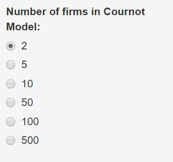
*In Demonstration $\PageIndex{2}$, the market inverse demand curve is $P = 200 - 2 \Sigma Q_{i}$ and $MC = 20$ for all firms.

Alternative Bertrand Version of the Oligopoly

In the Cournot model, firms compete by setting quantities. The Bertrand model is an alternative formulation of the oligopolists’ problem and differs in that the firms compete by setting prices instead. This model is named after Joseph Bertrand, a mathematician who is credited with formalizing this model. Again, to keep things simple, assume that there are two firms. Furthermore, assume that the products produced by each firm are identical. This permits us to take the example above and adapt it to the Bertrand framework.

If Firm A sets its price lower than Firm B’s price ($P_{A} < P_{B}$), then Firm A faces a direct demand function of

$Q_{A} = 100 - \dfrac{1}{2} P_{A}.$

If Firm A sets its price above Firm B’s price, then Firm A’s demand is

$Q_{A} = 0$

Finally, if Firm A’s price matches Firm B’s price ($P_{A} = P_{B}$), then consumers randomly choose to patronize Firm A or Firm B with equal probability. In this case, Firm A stands to get about half the market, so its demand is

$Q_{A} = 0.5(100 - \dfrac{1}{2}P_{A}).$

The demand facing Firm B is similarly structured. Firm B gets the entire market if $P_{B} < P_{A}$, sells nothing if $P_{B} > P_{A}$, and splits the market 50/50 with A if $P_{B} = P_{A}$. As before, assume that each firm faces a constant marginal cost of MC = $20.

The Bertrand Nash equilibrium outcome occurs where $P_{A} = P_{B} = MC$. In this case, profits to each firm are zero, and the oligopoly outcome is the same as that which would have occurred under perfect competition. Demonstration $\PageIndex{3}$ reflects the scenario just described and shows why.

Suppose that Firm A and Firm B have each chosen the monopoly price of $110. Each makes $2,025. This cannot be a Nash equilibrium because $110 is not the best price for Firm A given that Firm B charges $110. Firm A could undercut Firm B by charging a price of $80, in which case Firm A’s profits would go up to $3,600. Of course, Firm B would undercut Firm A and the process would continue until each firm’s price fell to its marginal cost of $20. This is the Bertrand Nash Equilibrium. No firm would cut below its marginal cost.

Demonstration $\PageIndex{3}$. Bertrand Duopoly

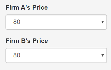
	Price	Quantity	Profits
Firm A	80.00	30.00	1800.00
Firm B	80.00	30.00	1800.00

The Folk Theorem

Both Cournot and Bertrand outcomes typify the prisoners’ dilemma because equilibrium outcomes do not maximize industry profits. In each case, there is a feasible outcome (sharing the market at the monopoly price and quantity) that makes firms better off than the Nash equilibrium profits.

Might firms be able to coordinate tacitly on a quantity less than the Cournot quantity or on a price higher than the Bertrand price? Suppose, for sake of argument, that Firm A and B are in Bertrand competition and each has matched the others price at $80. This price is above the Bertrand Nash Equilibrium price of $20 per unit, but it corresponds to the market price the firms would get at the Cournot Nash Equilibrium. If, in the current period, Firm A raises its price from $80 to $110, the monopoly price, how should Firm B respond? Pretend that you are Firm B. You might reason as follows:

If I keep my price at $80 and do not raise my price to match Firm A, I will have the entire market during this period. My profits will be $3,600. This is certainly better than $2,025 I would receive if I did match Firm A’s higher price.
However, if I do not match, I cannot expect that Firm A will not continue to keep its price high in the next period. When it sees that I have not matched its price increase and it loses market share, it will certainly cut is price back to $80 during the next period or possibly even lower. I will be back to getting $1,800 in profits (or possibly something worse).
If I do match Firm A’s price increase, Firm A will probably continue to keep its price high at $110. Thus I will be getting $2,025 each period as opposed to $1,800. Over the long-term, matching the price increase would pay off.

In this highly stylized example, the decision to match the price increase boils down to taking a one-time windfall of $3,600 (if Firm B does not match) or a $2,025 in profits in every period going forward (if Firm B does match).

The folk theorem states that for an indefinitely repeated prisoners’ dilemma (such as Bertrand) and provided that discount rates are not too high, an outcome preferable to the Nash equilibrium (e.g., a price above the Bertrand price) can be sustained over time. One way firms reinforce the folk theorem is to match their competitors’ pricing decisions tit-for-tat. Tit-for-tat means that one agent responds in kind to another. In the Bertrand example, Firm B plays tit-for-tat if it cuts (raises) its price whenever Firm A cuts (raises) its price. Firm B would want Firm A to know that it intends to play tit-for-tat in setting its prices. Thus, it might advertise to make sure Firm A is aware that it will face tit-for-tat retaliation in the event it decides to cut its price.

Many advertisements that you see send a subtle message to competitors that they can expect tit-for-tat retaliation in the event of a price cut. For example, consider the following Walmart advertisement: go to youtube.com. The advertisement is designed to make you feel like you will be getting the best price if you shop at Walmart and that the whole supply chain is organized to keep prices low. However, this add could also sends a subtle message to competing retailers. The message is as follows: If you cut your price, Walmart will match it. In other words, think carefully before making a price cut because Walmart will respond tit-for-tat!

Oligopolists may appeal to the folk theorem and avoid the prisoners’ dilemma inherent in the Cournot and Bertrand models provided certain conditions are met. The theorem itself mentions two conditions.

The first is that all firms expect the competitive interaction to continue indefinitely. The folk theorem works because future profits serve as an incentive not to undercut competitors today. If firms know that competition will be for this period and this period only, then there is no incentive not to undercut. Moreover, if firms know they will compete for a known and finite number of periods, the incentive not to undercut unravels. This is because all firms expect the others to undercut them in the last period, which means it would be best to undercut in the second-to-last period, which means it would best to undercut in the third-to-last period, and so forth. The folk theorem only works if firms expect to be in competition for the foreseeable future.
Another requirement is that discount rates not be too high. For the folk theorem to apply, future returns that result from not undercutting your competitor’s price must be large enough to offset the immediate gains you will receive if you do undercut a competitor. If discount rates are high, then returns in the future have less value today and the folk theorem is less likely to apply.

The rapidity with which firms can respond to price changes of competitors also affect whether the folk theorem can hold. If firms play tit-for-tat, then when one firm undercuts, it can expect retaliation by other firms. If it takes a long time for other firms to retaliate, then undercutting becomes more attractive regardless of the discount rate.

It also helps if firms are similar. This is because it is illegal for firms to collude to fix prices. There must be some price point that all firms can agree upon tacitly, without formally colluding to fix a price. The existence of such a point will be more likely if firms are reasonably similar in terms of costs and product characteristics.