If a seller can perfectly price discriminate, he or she is able to charge the buyer’s maximum willingness to pay for each unit. This is discriminatory because the price depends on the consumer’s willingness to pay not the cost of providing the product. If demand is downward sloping, the seller will charge a high price for the first unit purchased and progressively lower prices for additional units until willingness to pay reaches the seller’s marginal cost. By pricing in this manner, the seller leaves no consumer surplus. What would have been consumer surplus has been turned into profits. Perfect price discrimination is also called first-degree price discrimination.
To effectively employ first-degree price discrimination, the seller needs to know the demand curve of each individual. Fortunately for consumers, this is something that the seller is not likely to know. However, there are some sales situations where the seller may attempt to ascertain the consumer’s reservation price and charge him or her accordingly. One example is a car dealership. Most car buyers do not expect to pay the full sticker price. The sticker price is simply a reference point. The salesperson interacts with the buyer, attempts to ascertain his or her reservation price, and then charges accordingly. Thus, it is in your interest to not appear overly eager when buying new car.
Schemes that Approximate First-Degree Price Discrimination
Even though sellers are not likely to know the consumers’ demand schedules, there are pricing schemes that can come close to first-degree price discrimination. These can occur if consumer demands are very similar, i.e., each consumer has about the same demand for the product. Before explaining why, it is useful to emphasize a couple of points about the models used to understand these pricing schemes and some that will follow later in the chapter:
The models that follow use individual-level demands as opposed to the market demand. An individual demand schedule reflects the demand for a given consumer (or the demand from a given segment of consumers). The market demand is the sum of these individual demands.
It will be assumed that marginal cost is constant with volume. In addition to simplifying the analysis, a constant marginal cost is probably not unreasonable given output changes necessary to respond to demand at the scale of the individual consumer.
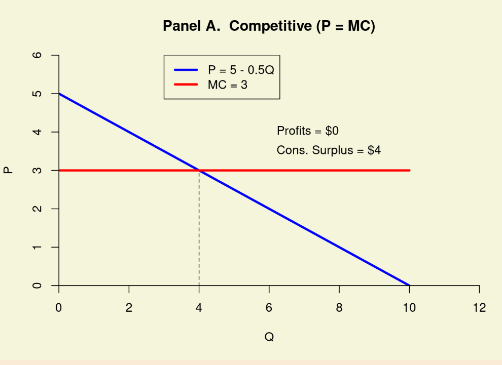
In addition to these two points, it is useful to revisit the difference between consumer surplus under a competitive (\(P= MC\)) outcome relative to the monopolist (\(MR=MC\)) outcome. Consider a case where all individual demand curves can be expressed in inverse form as
\(P = 5-0.5Q,\)
and marginal cost is given by MC=3MC=3.
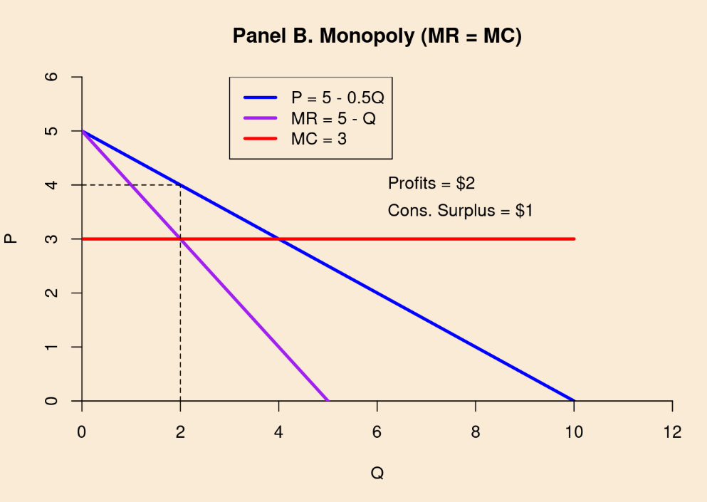
If the market is competitive (\(P=MC\)), each consumer buys four units at a price of $3 each and receives consumer surplus of $4. This is shown in Panel A of Figure 1. If, on the other hand, quantity is set so that marginal revenue from each consumer equals marginal cost (the monopolist’s solution), the monopolist gets economic profits of $2 from each consumer, $1 is left for each consumer as surplus, and $1 is lost because of the resource distortion inherent in the monopoly solution. This is shown in Panel B of Figure \(\PageIndex{1}\).
Figure \(\PageIndex{1}\): By pricing as a monopolist the firm can appropriate some but not all of the potentially available consumer surplus.
Could the firm do better then simply pricing as a monopolist? After all, the monopolist in this example leaves half of the potential surplus on the table. Specifically, $1 remains with the consumer and $1 goes away in the form of a dead-weight loss. It turns out that the answer to this question is yes. Because each consumer has the same demand curve, the firm can do much better. The firm can implement one of two pricing schemes:
Bundle the goods and sell bundles.
Charge an access fee that is equal to consumer surplus then set the price per unit equal to marginal cost.
Bundle Pricing
The seller that faced the consumers each with the individual demand curve in Figure 1 could sell four-unit bundles and charge a bundle price. The bundle price would equal to the consumer’s maximum willingness to pay for the four units, which is the entire area under the demand curve as we move from zero to four units. This is $16/bundle and is computed as the consumer surplus of $4 in Panel A of Figure 1 plus the $12 cost of producing the four-unit bundle.
With the bundle pricing scheme, the firm only offers bundles for sale. Consumers cannot buy individual units. They must buy bundles of four and pay the $16 price or not buy the product at all. The bundle price is set at the consumer’s maximum willingness to pay. No surplus is left for the consumer. In this example the bundle pricing scheme results in $4 in economic profits, double the profits that could be obtained by pricing as a monopolist.
Access Fees
Alternatively, the firm could charge an access fee of $4. Again, this is equal to the consumer surplus shown in Panel A of Figure \(\PageIndex{1}\). The price per unit is then set at MC or $3/unit. The consumer who pays the access fee is then able to purchase all he or she wants at $3/unit. Note, however, that the consumer will only purchase four units. His or her willingness to pay for additional units beyond four is less than the $3 price. In the end, the firm receives $16 from each customer (the $4 access fee and the $12 in product sales). Again the access-fee scheme results in profits of $4 from each consumer, which is double the profits of pricing as a monopolist. Some examples of access fees include all-you-can-eat buffets, cover charges at a bar or night club, and membership fees at a club store. In each of these situations the consumer pays up-front for access to a facility. Once in the facility, he or she can consume/purchase items at a fixed price (which could be zero in the case of an all you can eat buffet) and stops consuming once the willingness to pay for an additional consumption item exceeds the set price.