Evaluating the welfare effects with general equilibrium is the same as with partial equilibrium. First we determine the equilibrium solution, then we find the optimal solution, and last we compare the equilibrium to the optimal solution.
The previous section used an Edgeworth Box with a price vector to find the initial equilibrium solution. We know that shortages and surpluses swing the price line to and fro until it settles down where the plans of the two consumers are mutually compatible.
In this chapter, we use the Edgeworth Box to display the optimal solution. The price vector is removed because prices play no role in determining the optimal solution. Just as with partial equilibrium, we logically separate the equilibrium from the optimal solution. If the two agree, then we know we have a good result.
Optimality
STEP Open the Excel workbook EdgeworthBoxParetoOpt.xls, read the Intro sheet, then go to the EdgeworthBox sheet.
The workbook is quite similar to the EdgeworthBox sheet from the previous section, except there is no price or market position information. We are not interested in markets right now. We are focused on determining the optimal solution.
An omniscient, omnipotent social planner, OOSP, is charged with determining the optimal allocation, given the initial endowment.
With OOSP’s special powers, we can reallocate the initial endowment as we see fit. Each point in the box is an allocation, distributing the total amounts of the two goods to A and B. We can arbitrarily give and take from one person to the other, choosing any point in the box. What should we do?
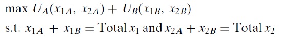
At first glance, it might seem that we would want to solve an optimization problem like this:
In other words, we could give consumers A and B the amounts of goods 1 and 2 that maximize the sum of the individual utilities subject to the total goods available.
This strategy suffers from a serious problem: We cannot make interpersonal utility comparisons. This brings us full circle to work we did at the very beginning of this book in the Theory of Consumer Behavior. Utility is ordinal, not cardinal. Monotonic transformations (that keep rankings intact) of utility are allowed. Utility has no meaning in terms of its units.
Thus, an optimization problem that aggregates individual utilities is invalid. It makes no sense to say that the utility of A is added to the utility of B to get a total utility. There are no common units with which to measure and add utility. You might as well say that you added three cars and four pencils and got seven carpencils.
There is, however, a way to judge and evaluate different allocations of goods to A and B. This is Pareto’s great contribution to welfare economics.
Pareto developed logical rules that enable us to get around the limitations of utility. His basic idea was that you can compare two allocations in terms of better or worse so you can make statements about one allocation compared with another. He invented a new vocabulary for his rules and today we use his name when we work with these rules.
Pareto knew we cannot add utility, but we might be able to compare two allocations and declare which one is better. We proceed by example, using the Excel workbook and Figure 18.6.
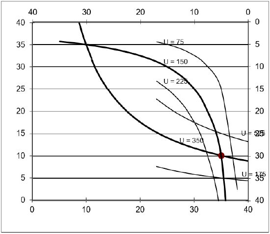
From the initial endowment point in Figure 18.6, suppose we consider the point (30,15) for A and (10,25) for B.
Figure 18.6 reproduces what is on your screen. The two thicker indifference curves going through the initial endowment are the starting point. They represent the benchmark satisfaction to which we will compare other allocations.
Figure 18.6: Edgeworth Box for Pareto criteria.
Source: EdgeworthBoxParetoOpt.xls!EdgeworthBox1.
From the initial endowment point in Figure 18.6, suppose we consider the combination of 30,15 for A and 10,25 for B.
STEP Click the button. A red point appears at that coordinate in the box along with a text box.
Is A better off at the new point compared with the initial endowment? How about B?
As the text box explains, although the indifference curves for A and B are not drawn through the red point, we know they exist because the indifference map is densethere is an indifference curve through every point in the box. If we draw an indifference curve for A through that point and it lies above the indifference curve that goes through the initial endowment, we know that A prefers 30,15 to the initial endowment.
In fact, indifference curves extend beyond the box in a northeast direction for A and southwest for B. The box just shows the total amounts available for exchange.
The same argument we made for A can be made for B. The only trick for B is to remember that you interpret the box from the top, right corner and B’s satisfaction increases as the indifference curves move farther away from the northeast corner in a southwesterly direction.
Because both A and B are better off at 30,15 than the initial endowment, we know that the 30,15 allocation is Pareto Superior to the initial endowment. We can also flip the statement to say that the initial endowment is Pareto Inferior to point 30,15.
Pareto Superior means that it is possible to make at least one person better off without making anyone else worse off. We make no claims as to how much better off. We do not use the units of utility at all. This is similar to how we first discussed satisfaction in the Theory of Consumer Behavior. We asked consumers to simply choose between one bundle and another. The same logic is being used here.
Consider another point that is 30,10 for A and 10,30 for B.
STEP Click the button.
As before, a red dot is placed on the chart and a text box appears. We want to compare the red dot to the initial endowment. Is A better off? How about B?
Because the point 30,10 is better for B, but worse for A, then this allocation is Pareto Noncomparable to the initial endowment because at least one person is made worse off. As soon as at least one person is made worse off, it is removed as a candidate for evaluation.
We certainly cannot evaluate these points by saying B’s utility goes up by more than A’s falls because utility is only ordinal. According to Pareto, we can never trade off a small decrease in satisfaction for one person for a large gain in satisfaction for one or many people because you cannot add up utility.
Now that we understand Pareto Superior and Pareto Noncomparable points, we can shade in all of the points that are Pareto Superior to the initial endowment. This is called the lens for reasons that will be obvious in a moment.
STEP Click the button.
Every point in the space between and including the two indifference curves going through the initial endowment is shaded red, representing the area of Pareto Superior points. With usually shaped indifference curves, this is a lens-shaped object.
We return to the first point, 30,15. It is, of course, inside the lens so it is Pareto Superior to the initial endowment, but does it have any points that are Pareto Superior to it?
STEP Click the button and then the 30,15 button.
The 30,15 point, like the initial endowment, has a whole set of points that are Pareto Superior to it. These points also form a lens, albeit smaller that the lens formed by the Pareto Superior points to the initial endowment, that stretch from the point 30,15 to where the two indifference curves intersect again.
Clearly, whenever indifference curves from A and B cross at a point, such as the initial endowment or 30,15, we can find Pareto Superior points in a lens from that starting point. What happens when the indifference curves are tangent?
STEP Click the (if needed) and buttons.
A red dot is shown on an indifference curve for B that is tangent to A’s highest displayed indifference curve. We will call this point of tangency between the indifference curves point PO1. This point PO1 is obviously Pareto Superior to the initial endowment since it is inside the lens.
But there is something special about PO1. It has a property that contains Pareto’s key idea: Does PO1 have any Pareto Superior points to it? No, it does not. Movement in any direction from point PO1 lowers someone’s satisfaction. There is no lens from point PO1.
Thus, we say that PO1 is a Pareto Optimal pointone that has no Pareto Superior points to it. You cannot make someone better off without hurting someone else. Pareto Optimal points are where we want to be!
It is important to note that there are an infinite number of Pareto Optimal points. Wherever the indifference curves are tangent, we are at a Pareto Optimal point.
The set of all Pareto Optimal points is called the contract curve. A minimalist version of a contract curve for an unknown (but well-behaved) pair of utility functions is displayed in Figure 18.7. A few indifference curves are displayed, but you should understand that every point on the contract curve is a point of tangency between two indifference curves. The sides of the box are not labeled, but you know how to read an Edgeworth Box.
Figure 18.7: The contract curve.
Pareto Optimal points are especially desirable because they ensure that there is no way to improve the allocation without harming someone. In other words, given the limitations of ordinal utility, we can say that we have wrung out as much gain as possible if we are at a Pareto Optimal point. Thus, from any given initial endowment, OOSP would want to reallocate the two goods so that the allocation is on the contract curve.
One drawback of the Paretian framework is that there are many Pareto Optimal points when starting from an arbitrary, non-Pareto Optimal point. There is no way to choose between Pareto Optimal points.
Mathematically, it should be clear that Pareto Optimal points occur only when \(MRS_A = MRS_B\). When this condition holds, the two indifference curves are tangent. This means we have a Pareto Optimal point and we are on the contract curve.
Pareto Optimality with Solver
One way to find Pareto Optimal points is to solve an optimization problem. It is not the silly, nonsensical “sum the utilities” objective function, however.
STEP From the EdgeworthBox sheet, open Solver.
Your Solver dialog box should look like Figure 18.8. Notice the \(UtilityB=Initial\_UtilityB\) constraint. We are going to maximize A’s utility without harming B. The constraint requires that B’s utility be the same as the initial utility. Thus, B will be indifferent between the new allocation and the initial endowment.
Figure 18.8: Solver parameters dialog box.
STEP Click to find an optimal solution to this problem.
Scroll down (if needed) to see the Edgeworth Box. We are at the top most (from A’s point of view) Pareto Optimal point. This point is on the contract curve.
What if we ran the same analysis, but maximized B’s utility subject to maintaining A’s utility constant? This is yet another Pareto Optimal point.
Some students want to make claims about points in the middle of the contract curve in the lens as being somehow better than the two extreme points, but the Pareto analysis does not allow for such distinctions.
The Contract Curve with Excel
STEP Proceed to the ContractCurve sheet.
It is set up just like the EdgeworthBox sheet, except A’s Initial Endowment cells (B18 and B19) have a formula, =ROUND(randomnv()*38+1,0).
This formula allows you to generate random initial endowments, then you can use Excel’s Solver to find a point on the contract curve from that initial endowment. You can use the “max A’s utility keeping B’s utility constant” or “max B’s utility keeping A’s utility constant” strategies. In the former case, you are finding the highest indifference curve of A that is tangent to B’s indifference curve that goes through the initial endowment. You are doing the reverse when you maximize B’s utility subject to A’s indifference curve that goes through the initial endowment.
STEP Click the button a few times to move the initial endowment point around the box. When you find one you like (it does not matter), find and record a point on the contract curve. Do this several times.
You are sampling points on the contract curve and this helps you learn how Pareto optimality works. Can you discover the shape of the contract curve?
STEP Change A’s preferences by setting cA to 0.5. Sample points on the contract curve (using the same method as in the previous step). What effect does this have on the contract curve?
To see the answers to these two questions (but first try to answer them on your own), click the button.
The First Fundamental Theorem of Welfare Economics
It is no exaggeration to say that we have reached the summit of this book. We are about to see the crowning achievement of economic theorya demonstration of the welfare effects of the market system in a general equilibrium framework.
With the Pareto criteria in hand, we are ready to judge the market allocation. Recall that the market uses prices to establish an equilibrium solution. Surpluses and shortages push the price vector to and fro until it settles down to its equilibrium solution. What can we say about the market’s solution?
We can say that it is Pareto Optimal! In fact, we can say that starting from any initial endowment, a market allocation mechanism yields a Pareto Optimal solution. This is the First Fundamental Theorem of Welfare Economics:
If preferences are well-behaved, a properly functioning market’s equilibrium solution is Pareto Optimal.
Figure 18.9 reproduces Figure 18.5 for your convenience. It is the canonical graph of general equilibrium analysis and shows the equilibrium solution from the Edgeworth-BoxGE.xls workbook. We know we have the equilibrium solution because there is a single, common tangency point. Consumer A maximizes by choosing that combination where he reaches the highest indifference curve subject to the constraint. Consumer B does the same.
Figure 18.9: Evaluating the market allocation.
Source: EdgeworthBoxGE.xls!EdgeworthBox1 with \(\frac{p_1}{p_2}=1\).
But it is immediately obvious, given our work in this section, that the market allocation is Pareto Optimal. There are no Pareto Superior points to it.
We can use the equimarginal principle to help explain this result. Each consumer is finding a point of tangency that obeys the mathematical condition, \(MRS = \frac{p_1}{p_2}\). From A’s perspective, we have \(MRS_A = \frac{p_1}{p_2}\). Similarly, B chooses that combination where \(MRS_B = \frac{p_1}{p_2}\). Unbeknownst to them, they are ending up at a point where \(MRS_A = MRS_B\).
In other words, by paying attention to prices and optimizing, the equilibrium generated by exchanging consumers is at the same time generating a Pareto Optimal solution. There is an invisible hand aspect to this in the sense that the consumers do not know and do not care about Pareto Optimality.
Geese fly in a V pattern over thousands of miles by draftingwind resistance is minimized by aligning one-self at angle to the goose ahead, instead of flying directly behind or next to a fellow goose. The geese are completely unaware that they are generating a V-shaped pattern. Consumers in a market are just like geesethey are completely unaware that they are solving a much bigger optimization problem.
Geese also synchronize their wing beats because they take advantage of updraft. If you watch a flock, it looks like they are coordinating their flapping. This was discovered recently (see Portugal, et al., 2014) and provides an excellent example of how economists see the market system.
With each agent following a simple rule, the system produces a pattern. In the case of the market, it is an incredible result that the market allocation is Pareto Optimal.
What can’t we say about the market allocation?
We certainly can’t say that it is fair. The market will grind to a Pareto Optimal point from any initial endowment. The Pareto logic takes the initial endowment as given. What if A starts out with much more than B? What if the market does not value B’s resources? The Pareto criteria have nothing to say about this. Economists have tried to include fairness in welfare analysis, but there is little consensus.
If there’s a First Theorem, there must be a Second Theorem, right?
If preferences are well behaved, a properly functioning
market can reach any Pareto Optimal point
if the appropriate initial endowment is provided.
The Second Fundamental Theorem says that you can use the market to reach any Pareto Optimal allocationthat is, any point on the contract curve. All you have to do is set the initial endowment appropriately, then let the market work its magic.
The last two problems in the Q&A sheet ask you to show that the Second Fundamental Theorem works.
That Markets Generate Pareto Optimal Solutions Is a Truly Fundamental Idea
This section marks the end of a long trek. We began with the Theory of Consumer Behavior and learned that consumers maximize satisfaction subject to a budget constraint. An important extension of this basic model utilizes an initial endowment instead of cash income.
In a Pure Exchange Model, we combine two optimizing consumers in an Edgeworth Box. Their interaction results in an equilibrium solution.
Using the Pareto criteria, we can compare allocations and determine which ones are Pareto Optimal. These are allocations that have no Pareto Superior points. The set of all Pareto Optimal points forms the contract curve.
Students struggle with the term Pareto optimality. Its definition, that there is no way to make someone better off without hurting someone else, can become a jumble of words with little real meaning. Here is the crucial idea: Pareto Optimality means no waste. The allocation at a Pareto optimal point cannot be improved upon (without harming someone). Thus, Pareto optimality means we have an unbeatable allocation.
The First Fundamental Theorem of Welfare Economics makes a powerful statement because it says that a properly functioning market yields a Pareto Optimal allocation. This is a highly desirable result.
It is also shocking because individual consumers have no idea they are participating in solving a resource allocation problem. Each consumer is simply maximizing utility subject to a budget constraint. Like geese that fly in a V, each consumer is responding to a signal (in the consumer’s case, prices) and then the interaction is producing the coordination.
Notice that the work here has said nothing about innovation or technological change. In fact, the analysis assumes constant technology and no new products. The analysis is completely static and based solely on the market’s ability to reach a Pareto Optimal solution in terms of allocating already produced goods in a pure exchange economy.
You might be wondering if all equilibria in an Edgeworth Box are Pareto Optimal? Absolutely not. The next section shows how the market can fail.
Exercises
Why do the Pareto criteria fail to provide a single point that is the best allocation?
What must be true about the exponents in the Cobb-Douglas utility functions for consumers A and B to generate a linear contract curve? Describe your procedure and explain your answer.
Use Word’s Drawing Tools to draw an Edgeworth Box with well-behaved preferences and a point Z, where the \(MRS_A > MRS_B\). Explain why point Z is not Pareto Optimal.
The contract curve (with cA = 0.5) can be transformed into a utility possibilities frontier, as shown in Figure 18.10. Where would point Z (from the previous question) be on this graph? Explain why.
Figure 18.10: A utility possibilities frontier.
Here in brief and incisive outline are the major ideas for which Pareto was later to become famous ... This slim volume is more readable and disciplined than most of the later elaborations, and serves well as an introduction to Pareto’s political sociology ... Pareto’s irony shows in his attack on elites that become humanitarian and tender-hearted rather than tough-minded.
Most economists know Pareto through his work on utility, General Equilibrium Theory, and the idea of Pareto Optimality, but Pareto grew disenchanted with “pure economics” (what we would call today economic theory) and turned to sociology. His most famous sociological work is Mind and Society (originally published in 1916 and first translated into English in 1935), in which he explains how the circulation of elites drives history.
See Vincent J. Tarascio, Pareto’s Methodological Approach to Economics (published in 1968) for a comparison of Pareto’s views on the scope and method of economics, especially as contrasted with Alfred Marshall. Whereas Marshall saw mathematics as a language, capable of being translated so nonmathematicians could understand, Pareto believed that “mathematics makes it possible to express relations between facts which are not possible with other facilities or ordinary language” (Tarascio, p. 106, footnote omitted). Pareto saw no need to translate heavily mathematical papers for the “literary economists.” Many of Pareto’s ideas on optimization and equilibrium were presented in prose form by Philip H. Wicksteed, Common Sense of Political Economy (first published in 1910) and available online at www.econlib.org/library/Wicksteed/wkCS.html.
On geese flying in a V and coordinating flapping, see Steven J. Portugal, Tatjana Y. Hubel, Johannes Fritz, Stefanie Heese, Daniela Trobe, Bernhard Voelkl, Stephen Hailes, Alan M. Wilson and James R. Usherwood (2014), "Upwash exploitation and downwash avoidance by flap phasing in ibis formation flight," Nature, 505, pp. 399–402, www.nature.com/articles/nature12939. My video, The Invisible Hand and the Market System, freely available at vimeo.com/econexcel/invisiblehand, has a clip of the authors explaining how the geese do it.


 button. A red point appears at that coordinate in the box along with a text box.
 button.
 button.
 button and then the 30,15 button.
 (if needed) and
  buttons.
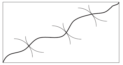 Figure 18.7: The contract curve.
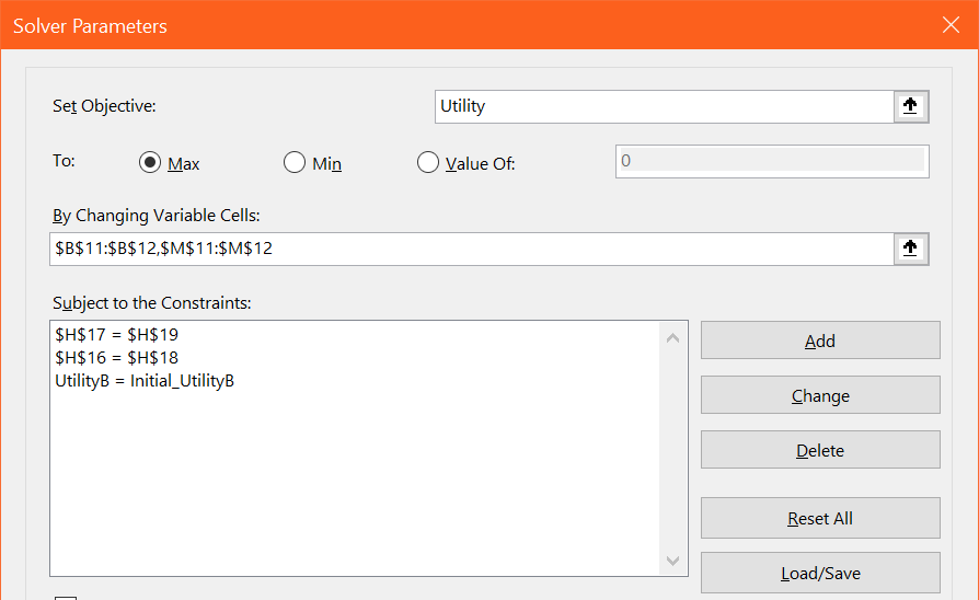 Figure 18.8: Solver parameters dialog box.
 to find an optimal solution to this problem.
 button a few times to move the initial endowment point around the box. When you find one you like (it does not matter), find and record a point on the contract curve. Do this several times.
 button.
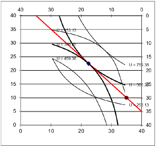
 Figure 18.10: A utility possibilities frontier.