Plot the labor and capital constraint to derive the production possibility frontier (PPF).
The production possibility frontier (PPF) can be derived in the case of fixed proportions by using the exogenous factor requirements to rewrite the labor and capital constraints. The labor constraint with full employment can be written as
\[ a_{LC}Q_C + a_{LS}Q_S = L \nonumber .\]
The capital constraint with full employment becomes
\[ a_{KC}Q_C + a_{KS}Q_S = K \nonumber .\]
Each of these constraints contains two endogenous variables: \(Q_C\) and \(Q_S\). The remaining variables are exogenous.
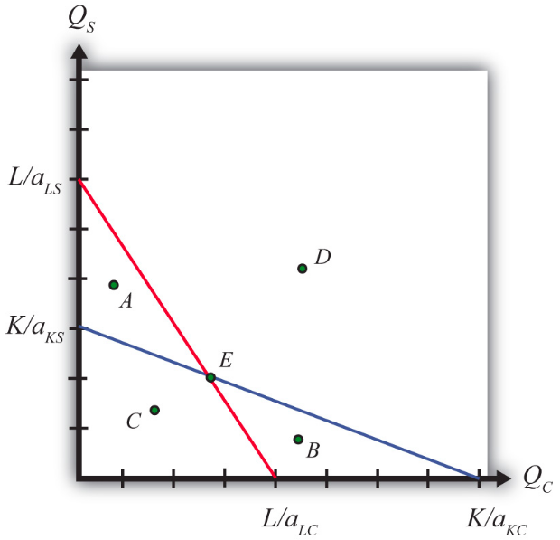
We graph the two constraints in Figure \(\PageIndex{1}\). The red line is the labor constraint. The endpoints \(\frac{L}{a_{LC}}\) and \(\frac{L}{a_{LS}}\) represent the maximum quantities of clothing and steel that could be produced if all the labor endowments were allocated to clothing and steel production, respectively. All points on the line represent combinations of clothing and steel outputs that could employ all the labor available in the economy. Points outside the constraint, such as \(B\) and \(D\), are not feasible production points since there are insufficient labor resources. All points on or within the line, such as \(A\), \(C\), and \(E\), are feasible. The slope of the labor constraint is \(-\frac{a_{LC}}{a_{LS}}\).
Figure \(\PageIndex{1}\): The Labor and Capital Constraints
The blue line is the capital constraint. The endpoints \(\frac{K}{a_{KC}}\) and \(\frac{K}{a_{KS}}\) represent the maximum quantities of clothing and steel that could be produced if all the capital endowments were allocated to clothing and steel production, respectively. Points on the line represent combinations of clothing and steel production that would employ all the capital in the economy. Points outside the constraint, such as \(A\) and \(D\), are not feasible production points since there are insufficient capital resources. Points on or within the line, such as \(B\), \(C\), and \(E\), are feasible. The slope of the capital constraint is \(-\frac{a_{KC}}{a_{KS}}\).
The PPF is the set of output combinations that generates full employment of resources—in this case, both labor and capital. Only one point, point \(E\), can simultaneously generate full employment of both labor and capital. Thus point \(E\) is the PPF. The production possibility set is the set of all feasible output combinations. The PPS is the area bounded by the axes and the interior section of the labor and capital constraints. Thus at points like \(A\), there is sufficient labor to make production feasible but insufficient capital; thus point \(A\) is not a feasible production point. Similarly, at point \(B\) there is sufficient capital but not enough labor. Points like \(C\), however, which lie inside (or on) both factor constraints, do represent feasible production points.
Note that the labor constraint is drawn with a steeper slope than the capital constraint. This implies \( \frac{a_{LC}}{a_{LS}} > \frac{a_{KC}}{a_{KS}} \), which in turn implies (with cross multiplication) \( \frac{a_{KS}}{a_{LS}} > \frac{a_{KC}}{a_{LC}} \). This means that steel is assumed to be capital intensive and clothing production is assumed to be labor intensive. If the slope of the capital constraint had been steeper, then the factor intensities would have been reversed.
Key Takeaways
The PPF in the fixed proportions Heckscher-Ohlin (H-O) model consists of the one point found at the intersection of the linear labor and capital constraints.
Only those output combinations inside both factor constraint lines are feasible production points within the production possibility set.
With clothing plotted on the horizontal axis, when the labor constraint is steeper than the capital constraint, clothing is labor intensive.
Exercise \(\PageIndex{1}\)
Jeopardy Questions. As in the popular television game show, you are given an answer to a question and you must respond with the question. For example, if the answer is “a tax on imports,” then the correct question is “What is a tariff?”
The description of the PPF in the case of fixed proportions in the Heckscher-Ohlin model.
The equation for the capital constraint if the unit capital requirement in steel is ten hours per ton, the unit capital requirement in clothing is five hours per rack, and the capital endowment is ten thousand hours.
The slope of the capital constraint given the information described in Exercise 1b. Include units.
The equation for the labor constraint if the unit labor requirement in steel is one hour per ton, the unit labor requirement in clothing is three hours per rack, and the labor endowment is one thousand hours.
The slope of the labor constraint given the information described in Exercise 1d. Include units.
The capital labor ratio in clothing given the information described in Exercise 1b and Exercise 1d.
The capital labor ratio in steel given the information described in Exercise 1b and Exercise 1d.