The model starts with the expenditure categories defined and measured in national accounts and described in Chapter 4. By the expenditure approach, GDP (Y) is the sum of consumption (C), investment (I), and exports (X), minus imports (IM). Then we can write:
\[\operatorname{GDP}(Y)=C+I+X-I M \label{6.1}\]
Expenditure as measured by national accounts is the sum of actual expenditures by business and households.
GDP(Y) is the national accounts measure of the sum of actual expenditure in the economy.
Aggregate expenditure (AE) is planned expenditure by business and households. The distinction between planned and actual expenditures is a key factor in explaining how the national income and employment are determined.
Aggregate expenditure (AE) is planned expenditure by business and households.
Induced expenditure
A simple short-run model of the economy builds on two key aspects of planned expenditure, namely induced expenditure and autonomous expenditure. First, an important part of the expenditure in the economy is directly related to GDP and changes when GDP changes. This is defined as induced expenditure. It is mainly a result of household expenditure plans and expenditure on imported goods and services embodied in those plans.
Induced expenditure is planned expenditure that is determined by current income and changes when income changes.
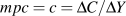
The largest part of consumption expenditure by households is induced expenditure, closely linked to current income. This expenditure changes when income changes, changing in the same direction as income changes but changing by less than income changes. The marginal propensity to consume (mpc=c) defines this link between changes in income and the changes in consumption they induce. The mpc is a positive fraction.
Marginal propensity to consume () is the change in consumption expenditure caused by a change in income.
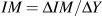
Household's expenditures on imports are at least partly induced expenditures that change as income and consumption expenditure changes. The marginal propensity to import (mpm=m) defines this link between changes in income and the changes in imports. The mpm is also a positive fraction because changes in income induce changes in imports in the same direction but by a smaller amount.
Marginal propensity to import () is the change in imports caused by a change in income.
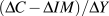
Because expenditure on imports is not demand for domestic output aggregate induced expenditure for the economy is determined by subtracting induced import expenditure from induced consumption expenditure to get induced expenditure on domestic output.
Induced expenditure (c–m)Y is planned consumption expenditures net of imports that changes when income changes.
The relationship between expenditures and national income (GDP) is illustrated in Table 6.1 using a simple numerical example and then in Figure 6.2 using a diagram.
Table 6.1 The effects of changes in GDP on consumption, imports and expenditure.
Consumption function:
C=0.8Y
Imports function:
IM=0.2Y
Y
Induced
Induced
Induced expenditure
0
0
0
0
50
40
10
30
100
80
20
60
75
60
15
45
The first row of the table illustrates clearly that if there were no income there would be no induced expenditure. The next two rows show that positive and increased incomes cause (induce) increased expenditure. The final row shows that a fall in income reduces expenditure. The induced expenditure relationship causes both increases and decrease in expenditure as income increases or decreases.
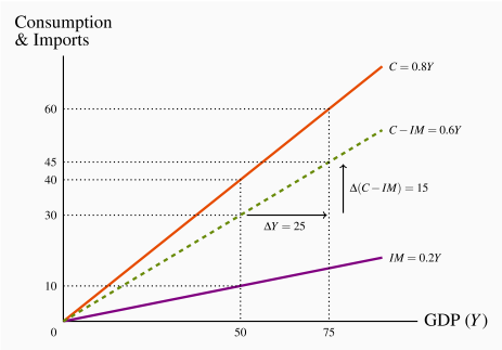
Figure 6.2 shows the same induced expenditure relationships in a diagram.
Figure 6.2 Induced expenditures
The slope of the C–IM line is: .
The positive slopes of the consumption and import lines in the diagram show the positive relationship between income and expenditure. A rise in income from 0 to 50 induces a rise in national expenditure from 0 to 30 because consumption expenditure increases by 40 of which 10 is expenditure on imports. If income were to decline induced expenditure would decline, illustrated by movements to the left and down the expenditure lines.
and .Figure 6.3 and size and stability of consumption share in expenditure GDP are strong evidence in support of that stability.
Figure 6.3 A Consumption Function for Canada, 1990–2016
Source: Statistics Canada, CANSIM Tables 380-0064 and 380-0065
Autonomous expenditure
The second part of GDP expenditure is where the real action lies. It covers the important changes in expenditure that drive the business cycles in economic activity. Autonomous expenditure (A), is the planned expenditure that is not determined by current income. It is determined instead by a wide range of economic, financial, external and psychological conditions that affect decisions to make expenditures on current output.
Autonomous expenditure (A) is planned expenditure that is not determined by current income.
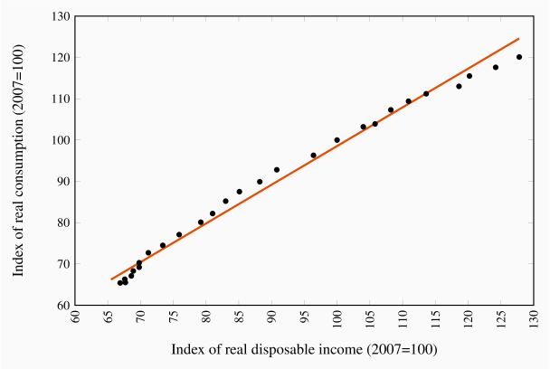
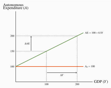
Consumption and imports have an autonomous component in addition to the induced component. But investment (I) and exports (X) are the major autonomous expenditures. Figure 6.4 shows the independence of autonomous expenditure from income. Unlike induced expenditure, autonomous expenditure does not change as a result of changes in GDP. The slope of the A line in the diagram is zero . However, a change in autonomous expenditure would cause a parallel shift in the A line either up or down. An increase in A is shown.
Figure 6.4 Autonomous expenditure
Investment expenditure (I) is one volatile part of aggregate expenditure. It is expenditure by business intended to change the fixed capital stock, buildings, machinery, equipment and inventories they use to produce goods and services. In 2014 investment expenditures were about 21 percent of GDP. Business capacity to produce goods and services depends on the numbers and sizes of factories and machinery they operate and the technology embodied in that capital. Inventories of raw materials, component inputs, and final goods for sale allow firms to maintain a steady flow of output and supply of goods to customers.
Firms' investment expenditure on fixed capital depends chiefly on their current expectations about how fast the demand for their output will increase and the expected profitability of higher future output. Sometimes output is high and rising; sometimes it is high and falling. Business expectations about changes in demand for their output depend on many factors that are not clearly linked to current income. As a result we treat investment expenditure as autonomous, independent of current income but potentially volatile as financial conditions and economic forecasts fluctuate. For example, the sharp drop in crude oil prices in late 2014 changed market and profit expectations dramatically for petroleum producers and for a wide range of suppliers to the industry. Investment and exploration projects were cut back sharply, reducing investment expenditure.
Exports (X), like investment, can be a volatile component of aggregate expenditure. Changes in economic conditions in other countries, changes in tastes and preferences across countries, changes in trade policies, and the emergence of new national competitors in world markets all impact on the demand for domestic exports.
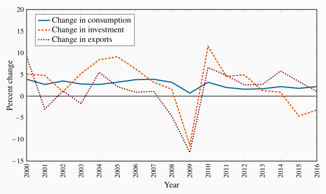
To illustrate this volatility in exports and in investment, Figure 6.5 shows the year-to-year changes in investment, exports, and consumption expenditures in Canada from 1999 to 2016. You can see how changes in investment and exports were much larger than those in consumption. This volatility in investment and exports causes short-term shifts in aggregate expenditure which cause business cycle fluctuations in GDP and employment. More specifically, the data show the sharp declines in investment and exports that caused the Great Recession in 2009 and even though these autonomous expenditures increased in 2010 those increases were not large or persistent enough to restore pre-recession levels of autonomous expenditure. Indeed investment expenditures have declined in 2015 and 2016.
Figure 6.5 Annual percent change in Real Consumption, Investment and Exports, Canada 2000–2016
Source: Statistics Canada, CANSIM Table 380-0064
The aggregate expenditure function
The aggregate expenditure function (AE) is the sum of planned induced expenditure and planned autonomous expenditure. The emphasis on 'planned' expenditure is important. Aggregate expenditure is the expenditure households and businesses want to make based on current income and expectations of future economic conditions. Expenditure based GDP in national accounts measures, after the fact, the expenditures that were made. These may not be the same as planned expenditure. Some plans may not work out.
Aggregate expenditure (AE) is the sum of planned induced and autonomous expenditure in the economy.
Aggregate expenditure (AE) equals the sum of a specific level of autonomous expenditure (A0) and induced expenditure [(c–m)Y] or in the simple notation introduced above:
(6.2)
Table 6.2 gives a numerical example of the aggregate expenditure function, assuming the marginal propensity to spend on domestic output (c–m)=0.5. It shows constant autonomous expenditure at each level of GDP, induced expenditure changing as GDP changes and aggregate expenditure as the sum of autonomous and induced expenditure at each level of GDP. Induced expenditure changes in the same direction as GDP which raises aggregate expenditure in rows 3 to 5 in the table but lowers aggregate expenditure in the last row when GDP falls.
Table 6.2 An aggregate expenditure function.
GDP (Y)
Autonomous
Induced
Aggregate
Expenditure
Expenditure
Expenditure
(A0=100)
(c–m)Y=0.5Y
AE=100+0.5Y
0
100
0
100
50
100
25
125
100
100
50
150
175
100
87.5
187.5
200
100
100
200
150
100
75
175
Figure 6.6 shows this aggregate expenditure function with a positive intercept on the vertical axis and positive slope. The positive intercept measures autonomous expenditure. The slope measures induced expenditure. Changes in autonomous expenditure would shift the AE function vertically, up for an increase or down for a decrease. Induced expenditures are usually assumed to be stable in the short run but if they were to change, as a result of change in marginal propensity to import for example, the slope of the AE function would change in the same way.
Figure 6.6 An aggregate expenditure function
The AE function has a vertical intercept equal to autonomous expenditure 100 and a slope of equal to the changes in expenditure induced by changes in Y.


 ) is the change in consumption expenditure caused by a change in income.
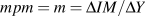 ) is the change in imports caused by a change in income.
 .
. and
and 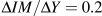 .
.
 . However, a change in autonomous expenditure would cause a parallel shift in the A line either up or down. An increase in A is shown.
 equal to the changes in expenditure induced by changes in Y.