Describe the traditional and modern neoclassical theories of utility maximization
Explain how to derive the demand curve using utility maximization
Explore criticisms of the neoclassical measure of welfare
Learn two competing solutions to the “paradox of value”
Analyze the complications that arise when preferences are endogenous
The Utilitarian Roots of the Theories
The theories that we will explore in this chapter have their roots in a philosophy called utilitarianism that developed in the nineteenth century. Utilitarianism is primarily a moral philosophy. According to its British founder, Jeremy Bentham (1748-1832), we ought to judge all social and economic policies according to the consequences that they carry for human happiness. If policies promote human happiness then they are morally right. If they diminish human happiness, then they are morally bankrupt. In other words, we ought to pursue the greatest happiness of the greatest number. Utilitarianism is mostly a normative theory, as defined in chapter 1. Its focus is primarily on what ought to be. John Stuart Mill is another famous thinker whose ideas on economics and politics utilitarianism greatly influenced, and the theory continues to have great influence among moral philosophers as well as economists.
By the late nineteenth century, many economists were beginning to reject the labor theory of value, arguably because its implications served critics of market capitalism more than it served its defenders. The notion that workers might be creating more value in production than they received in compensation was too threatening to those who wished to maintain the present social order. In its place, they discovered a theory of value that appeared to shift the focus back to the value that consumers obtain from consumption and away from labor content or cost of production. It was this discovery that gave rise to a school of economic thought that was so far removed from the classical economics of Smith and Ricardo that it was given the new title of neoclassical economics.
In the 1870s, three economists working independently co-discovered a concept that would form the basis of neoclassical microeconomics for the next century and a half. Leon Walras in France, William Stanley Jevons in Britain, and Carl Menger in Austria each developed the concept of marginal utility and identified an economic law to which they claimed all consumers are subject. They shifted the emphasis from the normative idea inherent in traditional utilitarianism (that we should pursue the greatest happiness of the greatest number) to a positive idea that economic agents, acting in a world of scarce resources, seek to maximize their own happiness. As economic agents go about maximizing their happiness, the economic law to which each is subject governs and determines their behavior in the marketplace.
The Concept of Utilityin the Traditional Theory of Utility Maximization
Before we define this economic law with precision, we must first define the concept of utility more carefully. The early neoclassical economists aimed to shift the focus of value theory back to the consumption side, but they did not wish to use the classical notion of use value. The use value of a commodity refers to the useful properties of a good or service. Utility, on the other hand, refers to the satisfaction that the user experiences in consumption.
One reason neoclassical economists define utility in terms of satisfaction is that they recognize that the experience of consumption is highly subjective. How useful the properties of a good or service are perceived to be depends on the user’s subjective mental experience. For that matter, an item might seem to an external observer to be useless. For example, in 1975 an entrepreneur had the idea to sell ordinary rocks as pets. These Pet Rocks had no function at all. They were simply good for a laugh. Nevertheless, the owner of the business became a millionaire before the item fell out of fashion. In addition, the good or service might not always appear to lead to pleasure. For example, if you go to the doctor for a shot, it might be painful rather than pleasurable. Nevertheless, on some level, you recognize that it is good for you to have it, and so you receive satisfaction despite the sting.
One of the strangest properties of utility according to the traditional theory of utility maximization is its quantifiable nature. Early neoclassical economists assumed that they could measure utility in terms of a standardized unit called utils. For example, you might obtain 25 utils of satisfaction from eating a bowl of cereal. This claim might seem silly, but remember that it is only an assumption for model building. Early neoclassical economists did not literally believe that satisfaction was a peculiar substance in the brain. Instead, they regarded it as a useful theoretical tool that would yield useful results. In other words, if we assume that satisfaction is measurable, does that assumption help us to explain and predict the behavior of individual consumers? Early neoclassical economists believed that it was so.[1]
The Law of Diminishing Marginal Utility
We next introduce a very important distinction between two key variables in the traditional theory of utility maximization: total utility and marginal utility. Total utility (TU) refers to the overall amount of satisfaction derived from the consumption of a good or service. For a certain period, we measure TU in utils. Marginal utility (MU) refers to the additional satisfaction obtained from the consumption of an additional unit of a good or service. We measure MU in utils per unit as follows:
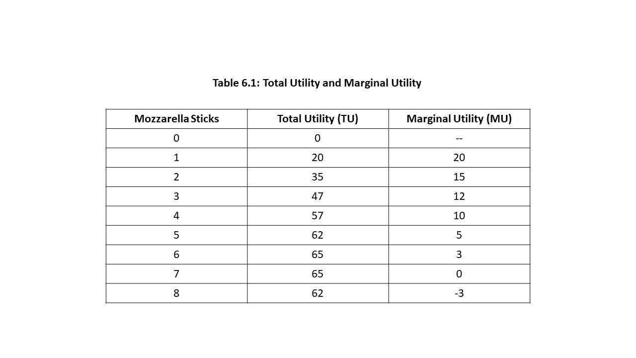
For example, six mozzarella sticks might give you a total utility of 65 utils, but the third mozzarella stick might only give you a marginal utility of 12 utils for that unit consumed. More generally, as an individual consumes more of a good, a clear pattern begins to emerge, argues the neoclassical economist. Table 6.1 shows what might happen to the total utility and marginal utility of a consumer as she consumes more mozzarella sticks.
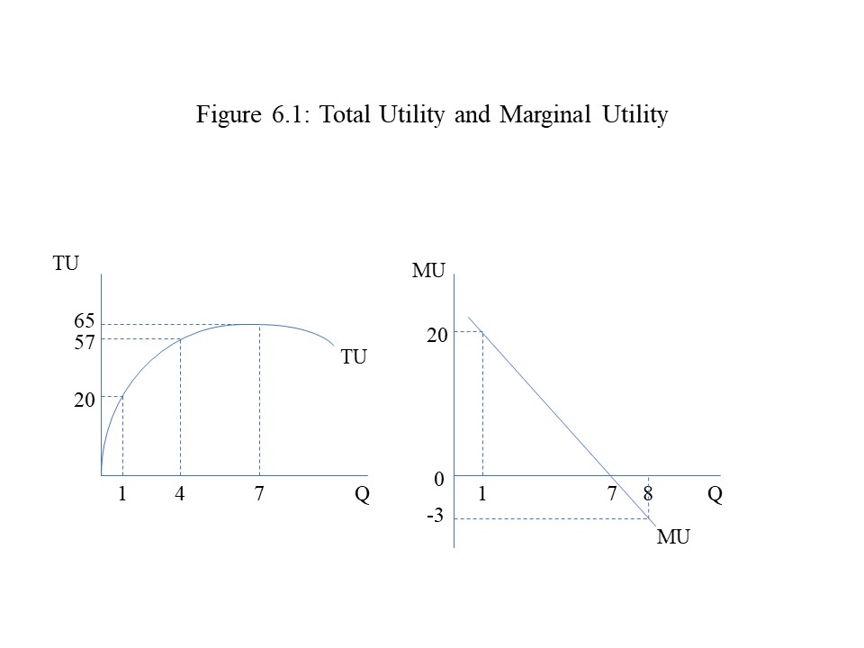
As the table indicates, as the consumer consumes more mozzarella sticks, the TU rises quite a bit even though it eventually begins to decrease. MU, on the other hand, falls from the beginning and eventually becomes negative. We can also graph these relationships as in Figure 6.1 where only a few of the points on each curve have been included.
These graphs of the TU and MU curves offer two different ways to visualize the law of diminishing marginal utility to which all individual consumers are subject, according to neoclassical economists. The law of diminishing marginal utility states that marginal utility declines as a consumer consumes more of a good. This reduction in MU is the result of the consumer attempting to satiate herself due to her consumption of the good. The marginal utility of each additional unit consumed is smaller and smaller until eventually an additional unit makes a negative addition to the total utility.Figure 6.1 shows that total utility rises as more of the good is consumed but at a decreasing rate. Eventually, total utility begins to fall as the consumer approaches satiation due to her consumption of the good.
It is worth noting the relationship between the two graphs. Mathematically, the slope of the TU curve is MU (=∆TU/∆Q). It should come as no surprise then that when total utility reaches its maximum, marginal utility equals zero utils per unit. That is, the slope of the TU curve is zero at the maximum point on the TU curve.
The law of diminishing marginal utility is perfectly compatible with the law of demand. If a consumer experiences a reduction in marginal utility as he consumes more of a good, then he will need a lower price to justify the purchase of an additional unit. That is, he will only be willing to purchase another unit if the price falls because that additional unit offers less satisfaction than the previous unit he consumed. Interestingly, the law of diminishing marginal utility also appears to be compatible with the discovery we made in chapter 5 that the price elasticity of demand falls all the way down a linear demand curve. It makes sense that a consumer would be less responsive to price changes at lower prices because those units correspond to lower marginal utilities.
The Traditional Theory of Utility Maximization
The law of diminishing marginal utility tells us how each consumer responds to the increased consumption of a good, but it does not tell us much about the consumer’s choices. Consumers generally consume more than one good. Consumers also must purchase these goods at constant prices and with limited incomes. To understand how much of each good a consumer will choose to purchase, we need a model to assist us with the analysis. To create an environment in which a single consumer makes decisions about how much of each good to purchase, we will assume that the consumer aims to maximize her total utility. It is also assumed that the consumer has complete preferences for the two goods available in the market and is subject to the law of diminishing marginal utility. Finally, the consumer faces a constant money income and constant prices for the two goods.
The statement that a consumer has complete preferences means that he knows exactly how many utils he will obtain from the consumption of a specific quantity of a good or service. In addition, the reader should notice the neoclassical entry point of given individual preferences and a given resource (or income) endowment. Overall, these assumptions are enough to make possible an analysis of the consumer’s utility maximizing choice.
We should begin with a simple example involving two goods. The consumer is trying to decide between the purchase of a television and a computer. Figure 6.2 captures the economic problem facing this consumer.
If the television will give the consumer 400 utils and the computer will give the consumer 800 utils, then one might conclude that the consumer should purchase the computer to maximize total utility. The problem with this line of reasoning is that it completely fails to consider the prices of the products. The price of the television might be $100 and the price of the computer might be $400. It turns out that the consumer will choose to purchase the television even though it gives the consumer less utility because the price is so much lower than the price of the computer.
To prove this point, we need to compare the marginal utility per dollar spent on each good (MU/$) by dividing the marginal utility of each good by its price. For example, the MU per dollar spent on the television is 400 utils/$100 or 4 utils per dollar spent. Similarly, the MU per dollar spent on the computer is 800 utils/$400 or 2 utils per dollar spent. Because the MU per dollar spent on the television is greater, the consumer will get more bang for her buck when she buys the television. We may state the general rule as follows:
The consumer will always purchase first the good that gives the higher MU per dollar spent.
We are now able to derive a more general result about utility maximizing behavior. Let us consider an example in which an individual is trying to decide how much of good X and how much of good Y to purchase. We will assume that the consumer’s income (M) is $35, the price of good X (PX) is $5 per unit, and the price of good Y (PY) is $3 per unit. We also assume that the consumer has clear preferences and so he or she knows the TU and MU for each quantity of the two goods consumed. Table 6.2 represents this information.
As the table shows, the consumer knows her preferences, and the law of diminishing marginal utility holds for each of the goods. In both cases, the MU falls as the consumer consumes more of the good. To calculate MU per dollar spent, we simply divide each MU by the price of the good in question.
The next question we wish to ask is how much of each good the consumer will choose given the income and the prices of the two goods. Because the consumer aims to maximize utility, the consumer will always select first the good that gives her the highest marginal utility per dollar spent. For example, assume that the consumer has an empty shopping cart and is trying to decide whether to purchase the first unit of good X or the first unit of good Y. Because the MU per dollar spent on the first unit of Y (= 15) is so much larger than the MU per dollar spent on X (= 5), the consumer will buy the first unit of Y. Next, the consumer must decide between the second unit of Y and the first unit of X. Because the eight utils per dollar spent on the second unit of good Y exceed the five utils per dollar spent on good X, the consumer will purchase the second unit of good Y. We need to keep track of expenditure as we proceed. Thus far, the consumer has spent $6.
Next, the consumer must decide between the third unit of good Y and the first unit of good X. In this case, either choice leads to five utils per dollar spent. The consumer will be completely indifferent in this case between the third unit of Y and the first unit of X. The reader might think that the consumer should choose the third unit of Y because it is cheaper but that would be a mistake. We already considered the fact that Y is cheaper than X when we divided the MU of each unit of each good by the appropriate price. Let us then assume that the consumer will choose the first unit of good X, bringing total expenditure to $11. Now the consumer must choose between the second unit of good X and the third unit of good Y. Because 5 > 4, the consumer will choose the third unit of good Y, bringing total expenditure to $14.
The next choice is between the fourth unit of Y and the second unit of X. Since 4 > 3, the consumer chooses the second unit of X. Expenditure has now reached $19. Next, the consumer is indifferent between the third unit of X and the fourth unit of Y because each yields 3 utils per dollar spent. If the consumer buys the fourth unit of Y, then total expenditure is up to $22. Now the consumer compares the MU per dollar spent on the fifth unit of good Y with the MU per dollar spent on the third unit of good X. Since 3 > 2, the consumer chooses to buy X, bringing total expenditure up to $27. Finally, the consumer is indifferent between the fourth unit of X and the fifth unit of Y. If the consumer chooses the fifth unit of Y, then total expenditure is $30. With the remaining $5, the consumer can buy the fourth unit of X because the sixth unit of Y has a negative MU and would reduce total utility.
With that final purchase, the consumer has purchased five units of good Y and four units of good X. It is the utility-maximizing combination of the two goods. In addition, the consumer has spent the entire $35 of income. Because we have been assuming that only the consumption of goods and services generates utility, it follows that the consumer must spend all income. If some income is not spent (i.e., if saving occurs), then utility cannot be at its maximum. The reader might object that individuals do choose to save. Neoclassical economists do analyze saving from a microeconomic perspective, but it involves a utility maximizing choice between present and future consumption rather than between two present goods.[2]
One other major result that deserves special attention is the fact that the MU per dollar spent on goods X and Y are the same when the consumer is maximizing utility. The final unit of each good yields 2 utils per dollar spent. It is possible to construct an example where the marginal utilities per dollar spent on each good are only approximately equal due to the consumer running out of money before the equality is reached. Nevertheless, the point remains that the consumer will continue to move back and forth between the two goods until the marginal utilities per dollar spent are nearly, if not exactly, equal. Excluding possible exceptions, we can sum up as follows:
The consumer maximizes utility when the marginal utilities per dollar spent are the same for both goodsand all income is spent.
Algebraically, it is possible to write this condition as follows:
Furthermore, if all income is spent and , then the consumer should buy more X and less Y. As more X is purchased, the MU of X falls due to diminishing marginal utility. Similarly, as less Y is purchased, the MU of Y rises due to diminishing marginal utility. These changes will continue until the marginal utilities per dollar spent are the same for the two goods.
Similarly, if all income is spent and , then the consumer should buy more Y and less X. As more Y is purchased, the MU of Y falls due to diminishing marginal utility. Similarly, as less X is purchased, the MU of X rises due to diminishing marginal utility. These changes will continue until the marginal utilities per dollar spent are the same for the two goods.
The Traditional Derivation of the Individual Demand Curve
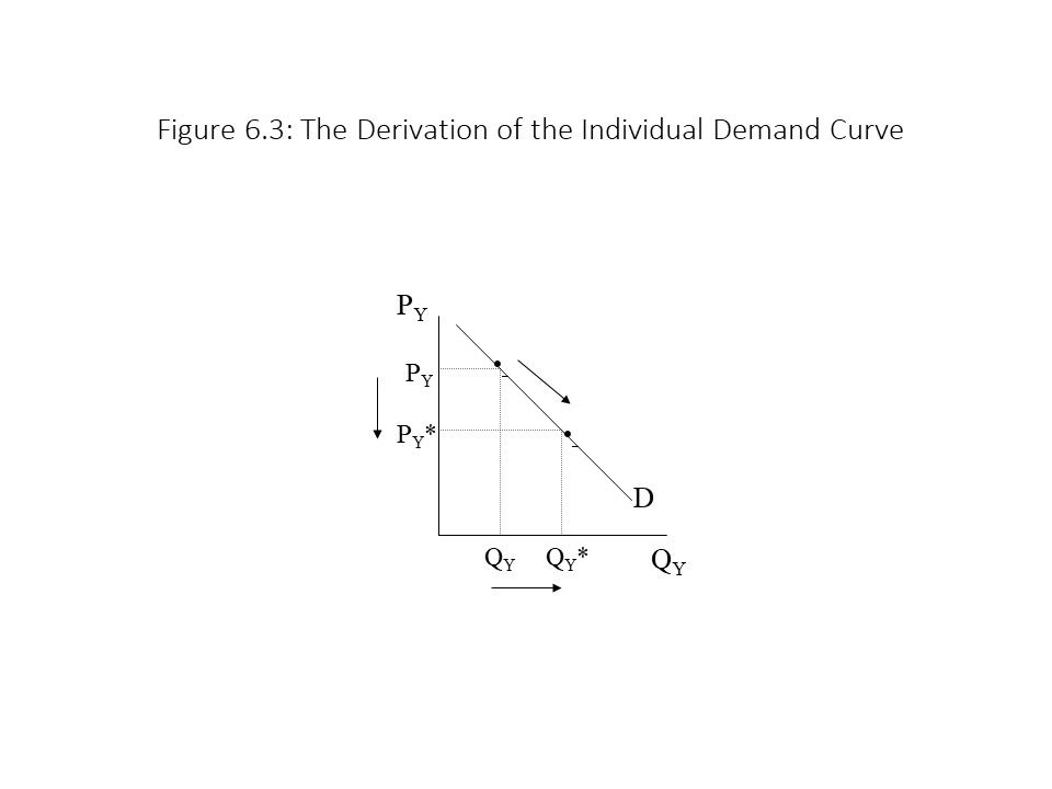
The utility maximizing condition described in the last section can be used to derive the individual demand curve. That is, we can gain a deeper understanding as to why the individual demand curve slopes downward when we think in terms of utility maximizing behavior. Suppose, for example, that the price of good Y declines. The law of demand states that the quantity demanded of Y will rise, other things the same. This situation is depicted in Figure 6.3.
Assume that the consumer is maximizing utility at the original price of PY. In other words, the initial condition when all income is spent is the following:
Now suppose that PY declines to PY*. It follows that:
Because the MU per dollar spent on good Y is greater than the MU per dollar spent on good X, the consumer will purchase more Y. Because the price of good Y fell and the quantity demanded of good Y rose, we can conclude that the demand curve slopes downward. It is worth noting that the increase in the quantity demanded of Y will eventually cease (when Q reaches QY*) because the diminishing marginal utility of Y will restore the equality between the two marginal utilities per dollar spent.
The Paradox of Value
The traditional theory of utility maximization also helps to resolve a paradox in the history of economic thought. A paradox is a statement that appears to be false but that contains an element of truth. The paradox of value refers to the fact that many goods, like diamonds, appear to be not very useful even though they have high prices. Similarly, the most useful goods, like water, often have the lowest prices.
The classical economists, like Smith and Ricardo, believed that they had successfully found the solution in the labor theory of value. That is, diamonds have a high price because they require a lot of labor time for their production. Similarly, water has a low price because it requires very little labor time for its production.[3]
Early neoclassical economists in the 1870s offered a different solution to the paradox than that which the classical economists offered. Their discovery of the marginal utility concept allowed them to develop a different solution to the paradox that emphasized consumer satisfaction rather than production cost. Specifically, they pointed out that the proper resolution to the paradox requires the distinction between total utility and marginal utility. That is, goods that most people consider to be useful, like water, generate a great deal of total utility for consumers. The marginal utility of the last unit consumed, however, is very low due to the law of diminishing marginal utility and the fact that so many units are consumed. It is the marginal utility of the last unit consumed that governs its price, according to this solution. In other words, the low MU of water explains its low price.
On the other hand, goods that most people regard as relatively useless, like diamonds, do not give consumers a great deal of total utility. The marginal utility of the last unit consumed, however, is very high due to the law of diminishing marginal utility and the fact that relatively few units are consumed. In this case, it is the high MU of diamonds that explains its high price.
We can also graphically represent the marginal utility solution to the paradox of value as shown in Figure 6.4.
The top graphs in the figure show that the total utility obtained from the consumption of water is very high due to the large volume consumed. The marginal utility of the last unit consumed is very low for that same reason. The bottom graphs in the figure show that the total utility obtained from the consumption of diamonds is very low because of the small amount consumed. For the same reason, the marginal utility of the last diamond consumed is very high. The reader should also observe the straight lines that are just tangent to the TU curves at the quantities consumed. The slopes of the tangent lines represent the marginal utilities. The relatively flat tangent line in the top left graph indicates a low marginal utility. The relatively steep tangent line in the bottom left graph indicates a high marginal utility.
Table 6.3 summarizes all the information in this section, including the paradox of value itself as well as the classical and early neoclassical solutions to the paradox.[4]
Criticisms of the Neoclassical Measure of Welfare
The concepts of consumers’ surplus and producers’ surplus that are discussed in Chapter 3 are presented as being logically consistent with the rest of neoclassical microeconomic theory. The concepts, however, are subject to two serious criticisms that can only be understood once we have a firm grasp of the theory of utility maximization.
The first major criticism is that the concepts implicitly assume a constant marginal utility of money. For example, suppose that I am willing and able to pay $5 for an ice cream sundae, but I only need to pay the market price of $2. I enjoy a consumer surplus of $3. Suppose further that I purchase a second ice cream sundae for $2 and that I am willing and able to pay $4 for the second one. I enjoy a consumer surplus of $2 on the second one that I purchase. My total consumer surplus is $5 (= $3+$2). This measure of my welfare only makes sense if the marginal utility of money is constant for me. That is, if the law of diminishing marginal utility applies to money, then the first dollar of consumer surplus that I receive will contribute more to my welfare than the last dollar that I receive. In other words, the yardstick by which we measure welfare must remain the same for consumers’ surplus to be regarded as an internally consistent measure of consumers’ welfare. The same criticism applies to producers’ surplus.
The second major criticism is that the concepts also implicitly assume that the marginal utility of money is the same for all buyers and sellers. This criticism becomes relevant when we attempt to aggregate the surpluses of different individuals. For example, suppose that my consumer surplus is a total of $75 and your consumer surplus is also $75. If we add our surpluses together, we obtain a total of $150. What if my marginal utility of money is much higher than your marginal utility of money? In that case, my surplus should count more in the aggregate measure than your surplus, but in this case, our surpluses contributed equally to this measure of consumer welfare. Both criticisms raise serious problems that have been recognized by neoclassical economists. Despite the difficulties, the concepts are still used and students are rarely encouraged to critically reflect on the problems inherent in the use of this welfare measure.
The Modern Theory of Utility Maximization
As we have seen, the early neoclassical economists assumed that utility was quantifiable and measurable. When utility can be quantified and measured, it is called cardinal utility. During the twentieth century, neoclassical economists realized their theory would be stronger if they abandoned an assumption as strict as this one. Their effort to rid consumer theory of this strict assumption is a good example of the application of a philosophical principle known as Ockam’s Razor. According to this principle, the strongest theory is the one based on the simplest assumptions, other things the same.
This principle has been applied in many contexts, including in the natural sciences. For example, during the nineteenth century, Charles Darwin developed the theory of natural selection to explain how organisms adapt to their natural environments over long periods of time. According to Darwin, random genetic mutations cause variations in the physical characteristics among the members of a species. Those members that develop the most advantageous characteristics for survival will thrive and reproduce. Those members with the least advantageous characteristics will die and fail to reproduce. As a result, the most advantageous characteristics are passed down and the least advantageous characteristics disappear from the species.
A little-known fact among non-scientists is that a competing theory of evolution also existed in the nineteenth century. According to a French anatomist by the name of Lamarck, the members of a species acquire advantageous characteristics during their lifetimes in response to their specific environments. For example, a giraffe stretches its neck to reach leaves further up on a tree, and thus acquires a longer neck, which it then passes down to its offspring. This claim, that an organism acquires traits that alter the genetic material passed down to its offspring, is an assumption of Lamarck’s theory that is much more complicated than Darwin’s assumption that random genetic mutations are the source of the advantageous characteristics. Because Darwin’s theory was based on a simpler set of assumptions, it was adopted and Lamarck’s theory was rejected. It should be emphasized that Darwin’s theory was not proven once and for all. It was accepted as the best theory due to the application of Ockam’s Razor.
Similarly, neoclassical economists aimed to replace the less plausible assumption of quantifiable satisfaction with a simpler assumption. That is, they rejected cardinal utility and replaced it with a different kind of utility called ordinal utility in their models of consumer behavior. The ordinal utility concept implies that consumers receive satisfaction from the consumption of goods, but they are only able to create a ranking among alternative commodity bundles (i.e., combinations of the goods).
For example, bundle 1 may consist of 2 apples and 1 banana whereas bundle 2 may consist of 1 apple and 2 bananas. If we use the notion of ordinal utility, then a consumer can only say one of three things: 1) Bundle 1 is preferred to bundle 2; 2) bundle 2 is preferred to bundle 1; or 3) bundles 1 and 2 are equally preferred (i.e., the consumer is indifferent between the two bundles).
On the other hand, if we use the concept of cardinal utility, then it would be possible to state that bundle 1 creates 10 utils for the consumer and bundle 2 creates 5 utils for the consumer. In that case, bundle 1 is not only preferred to bundle 2, but it is exactly twice as preferred as bundle 2. That is, the cardinal utility assumption allows us to state how much more preferred one bundle is than another. With the ordinal utility assumption, it is only possible to state that one bundle is more preferred than another, but it is impossible to state how much more preferred that bundle is.
The Implicit Ideological Significance of the Ordinal Utility Assumption
Before we explore the modern theory of utility maximization at greater length, we should pause to consider the implicit ideological significance of the ordinal utility assumption. It will not be immediately obvious to the uninitiated reader what role this assumption plays in neoclassical theory, but it can be explained easily enough if one is willing to be direct about it.
If cardinal utility is assumed, then satisfaction is quantifiable. Suppose person A has $1 million and person B has only $10,000. Suppose also that the MU of an additional $10,000 for person A is 10 utils, but the MU of an additional $10,000 for person B is 500 utils. If the law of diminishing marginal utility holds, then this assumption seems to make sense. That is, the relatively poor individual values the additional $10,000 much more than the wealthy individual. It seems that we might be able to make a case for a redistribution of wealth from person A to person B strictly on efficiency grounds. Society will enjoy a net gain of about 490 utils due to the transfer.[5]
On the other hand, if we assume ordinal utility, then all we can assert is that both individuals will prefer the larger sum ($1,010,000 for person A and $20,000 for person B) to the smaller sum ($1,000,000 for person A and $10,000 for person B). We cannot say how much more each person prefers the larger sum to the smaller sum. As a result, it is impossible to conclude that a redistribution of money will lead to a net welfare gain. With ordinal utility, interpersonal utility comparisons are impossible. That is, who is to say that the individual with $1 million will value an additional $10,000 less than the individual with only $10,000? Because we lack a common yardstick for the measurement of satisfaction, we cannot justify the redistribution of wealth on efficiency grounds. If any argument is to be made for the redistribution of wealth, it must appeal to our desire for greater equality or some standard of fairness. For those wishing to limit government redistributions of wealth and income, the ordinal utility assumption is a powerful one.
The Assumptions of the Modern Theory of Utility Maximization
Just as in the case of the traditional theory, it is necessary to specify the conditions in which the consumer makes decisions with the goal of maximizing utility. It is again assumed that the consumer is choosing between two goods, X and Y. The consumer also possesses a fixed money income (M) and faces a constant price for good X (PX) and a constant price for good Y (PY). The consumer also has given individual preferences. The only major difference between the two theories is that the consumer’s preferences must be represented differently because in the modern theory, utility is not quantifiable.
Budgets, Preferences, and Utility Maximization
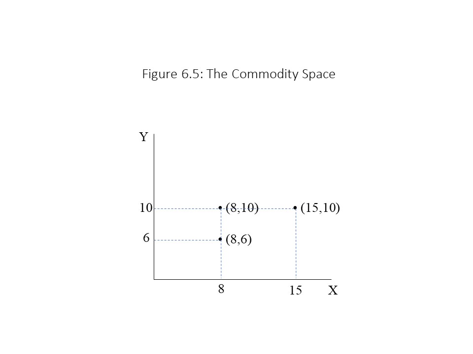
To graphically represent the modern theory of utility maximization, we will be working in a two-dimensional space called the commodity space. An example is shown in Figure 6.5 where the quantities of goods Y and X are measured on the vertical and horizontal axes, respectively.
Each point in the commodity space represents a commodity bundle, or a combination of the two goods. For example, the ordered pair (8, 6) represents a commodity bundle that includes 8 units of good X and 6 units of good Y.
Our purpose is to determine which of the affordable bundles in the commodity space maximizes the consumer’s utility. We will approach this problem in three parts. First, we will determine the set of all affordable bundles in the commodity space for a given income level and prices. Second, we will explain how preferences may be represented when utility is ordinal using an analytical device designed for this purpose known as indifference curves. Finally, we will bring together the consumer’s budget with her preferences to determine the utility maximizing commodity bundle.
In terms of the consumer’s budget, we know that the money income and the prices of the two goods are fixed. Let’s first see if we can determine all the commodity bundles that require the consumer to spend all her income. In other words, let’s assume the following condition:
If the consumer spends the entire money income, then no saving exists. This same condition can be written symbolically in the following way:
The overbars in the equation indicate that the prices and income are constant. Only the quantities of goods X and Y are variables in the equation because only they can be influenced by the consumer’s choices. To graph this equation in the commodity space, we need to solve for the variable on the vertical axis. If we solve for Y, we obtain the following result (omitting the overbars):
This equation is in slope-intercept form and so it is now possible to graph this equation as a straight line in the commodity space. The vertical intercept is constant and is equal to M/PY. The slope is also constant and is equal to –PX/PY. The horizontal intercept can also be determined by setting Y equal to 0 and solving for X as follows:
All these results are captured in Figure 6.6:
In economic terms, the vertical and horizontal intercepts refer to the maximum quantities of Y and X, respectively, that can be purchased if the consumer spends the entire money income on one or the other good. Each of the other points on the budget line represents a commodity bundle that requires the consumer to spend the entire money income. Bundles below the budget line are affordable but do not require the expenditure of the entire income. For example, if a consumer began at a bundle on the budget line and reduced the amount of Y by a small amount, then some income would be left over. Hence, that bundle would be affordable but would not require the expenditure of the entire income. All the bundles on the budget line and those below the budget line are affordable and are therefore considered part of the consumer’s budget set. Any bundle above the budget line is not affordable because the consumer would need more income than she possesses to make that purchase.
The slope of the budget line is also important and can be written as follows:
The slope of the budget line represents the ability of the consumer to trade off one good for another in the marketplace at the current prices. That is, if the consumer would like to purchase one more unit of X, she will have to give up –PX/PY units of Y. The reader might be thrown off by the fact that PX is in the numerator and PY is in the denominator. It should be remembered that the units in which price is measured, however, are $ per unit. Therefore, PX is measured in $/X and PY is measured in $/Y. The division yields Y/X, which are the correct units attached to the slope of the budget line.
To make this discussion a bit more concrete, let’s consider a numerical example. Suppose M = $20, PX = $5, and PY = $4. We can write the budget equation and then solve for Y as follows:
This budget equation may be graphed as in Figure 6.7.
The reader should notice that the intercepts may be obtained quickly since M/PX = 4 and M/PY = 5. The slope may also be determined quickly because –PX/PY = –5/4 = –1.25. That is, if the consumer wishes to increase the consumption of X by one unit, then he must give up 1.25 units of Y.Figure 6.8 shows what will happen if changes occur in M, PX, or PY.
As the figure shows, a rise in M will increase both intercepts proportionately, leading to an outward, parallel shift of the budget line. More income thus makes more bundles affordable. Similarly, a rise in the price of X leads to a rotation inwards of the budget line because the vertical intercept is unaffected. In this case, the budget set contracts because the higher price of X makes fewer bundles affordable. Finally, a rise in the price of Y also makes the budget line rotate inwards because the horizontal intercept is unaffected. The contraction of the budget set indicates that fewer bundles are affordable. The reader should work through what will happen when the consumer’s income or the prices of the goods fall.
We now turn to the representation of preferences within the modern theory of utility maximization. The key analytical tool for this purpose is a device called an indifference curve. It is defined as follows:
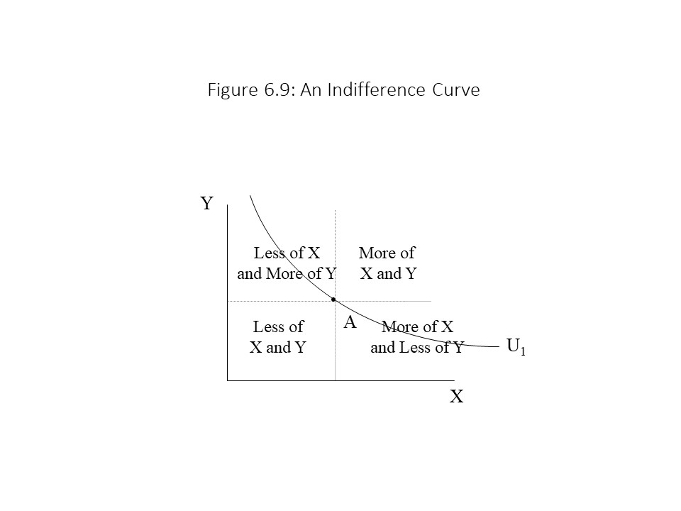
An indifference curve through commodity bundle A is a line drawn through all the commodity bundles that the consumer considers to be equally satisfying in relation to commodity bundle A.
An example of an indifference curve is given in Figure 6.9.
All the bundles along indifference curve, U1, are equally preferred to all other bundles on that same indifference curve. It is also possible to identify regions that have more of both goods relative to bundle A, less of both goods relative to bundle A, more Y and less X relative to bundle A, and less Y and more X relative to bundle A.
Our next task is to explain why the indifference curve through bundle A slopes downward as well as why it is bowed away from the origin (as opposed to a straight line or having some other shape). The downward slope indicates that the consumer is willing to trade off some of good Y for more of good X and vice versa. For example, if the consumer begins at bundle A, and she loses some of good Y, then the only way to restore her to the U1 level of satisfaction is to increase her consumption of good X. Therefore, the indifference curve slopes downward.
The fact that the indifference curve is bowed towards the origin indicates something significant about the willingness of the consumer to trade off one good for another. To clarify this point, we will refer to the slope of the indifference curve as the marginal rate of substitution (MRS). Figure 6.10 shows clearly that the slope is very steep at low levels of X and becomes very flat at high levels of X.
As the figure shows, when the MRS is – 5 (approximately) the consumer is willing to sacrifice 5 units of Y for one more unit of X. When the MRS is – 3 (approximately) the consumer is willing to sacrifice 3 units of Y for 1 more unit of X. Finally, when the MRS is – 1 the consumer is willing to sacrifice only 1 unit of Y for 1 more unit of X. Clearly, as the consumer consumes more X, the amount of Y he is willing to sacrifice to obtain another unit of X becomes smaller and smaller. In other words, X is becoming less valuable to the consumer as more of it is consumed. Although this result sounds a great deal like the law of diminishing marginal utility, it was obtained without the use of cardinal (quantifiable) utility. The only reason that we know the consumer values additional units of X less as more of it is consumed is that he is willing to give up less and less Y for those additional units. Diminishing marginal rate of substitution is the phrase we can use to refer to this tendency of the MRS to fall (in absolute value) as more X is consumed.Figure 6.11 shows one example of an indifference map.In the figure, a few commodity bundles have been labeled. Is it possible to identify the consumer’s ranking of these bundles? It is so long as we assume that more of both goods is always preferred to less of both goods. If we make this assumption, then it follows that any commodity bundle on a higher indifference curve must be preferred to any bundle on a lower indifference curve. In this case, W and A are equally preferred. W and A are strictly preferred to C and H, which are equally preferred to one another. Finally, Z and G are equally preferred to one another, and they are less preferred than C and H. We are free to state that W and A give the consumer the most utility, but since we are using an ordinal notion of utility, this statement only means that they are the most preferred bundles in the ranking.Figure 6.12 shows a consumer’s budget line and two of her indifference curves.
We want to determine what the utility maximizing commodity bundle is. We can begin by narrowing down the possibilities very quickly. The bundle that maximizes utility must be on the budget line. If it is not, then the consumer will have income left over. Because only the consumption of goods generates utility, the consumer cannot be maximizing utility unless she is consuming on the budget line.
Suppose we consider a bundle on the budget line such as bundle B. Because this bundle is on the budget line, we know that all income is being spent. Does it maximize utility though? It does not. The reason is that the indifference curve through bundle B (U1) is lower than the indifference curve through bundle A (U2). Therefore, the consumer prefers bundle A to bundle B. Because bundle A is affordable, the consumer should buy less Y and more X until she reaches bundle A. Similarly, if the consumer is consuming bundle C, then it is possible to reach the higher indifference curve by reducing her consumption of X and increasing her consumption of Y until she reaches bundle A where she consumes X* units of X and Y* units of Y.
At bundle A, the consumer is maximizing utility because all income is spent, and it is not possible to reach a higher indifference curve by choosing a bundle within the budget set. At that bundle, the budget line is tangent to the highest indifference curve passing through the budget set. Mathematically, the slope of the budget line must equal the slope of the indifference curve. We can express this condition symbolically as:
This utility maximizing condition may be written another way as well. Let’s first recall that total utility remains constant as we move along an indifference curve. That is, ∆TU = 0. When moving along the indifference curve, we can assume that the consumer reduces her consumption of good Y (by ∆Y) and increases her consumption of good X (by ∆X). The change in total utility can now be divided up into the loss of utility from the reduced consumption of Y plus the gain in utility from the increased consumption of X. That is:
If we solve the above equation for ∆Y/∆X, we obtain the following result:
Even though utility is not measurable in the modern framework, the utils cancel out in the fraction and so the MRS is a ratio of the change in Y to the change in X. We include the marginal utilities because this new manner of expressing the MRS allows us to write the utility maximizing condition in the following way:
By rearranging the terms and eliminating the negative signs, we obtain the same result that we obtained in the traditional theory of utility maximization.
In other words, the marginal utilities per dollar spent must be the same for both goods for utility to be maximized. This result was a remarkable outcome for neoclassical economists. They obtained precisely the same result that they had obtained with the traditional theory, but they did so without the less realistic assumption of cardinal utility. Other things the same, the theory with the simplest assumptions became the chosen theory. Ockam’s Razor had been successfully applied.
The ModernDerivation of the Individual Demand Curve
The modern theory of utility maximization also allows us to derive the downward sloping individual demand curve. Figure 6.13 provides the graphical analysis by which the demand curve is derived within a utility maximizing framework.
In Figure 6.13, the price of good X rises from P1 to P2, causing a rotation inward of the budget line. The consumer moves from one utility maximizing point to another. In this case, he reduces the quantity demanded of X from X1 units to X2 units. The result is a movement up the individual demand curve. Because the consumer moves to a lower indifference curve, it is apparent that the consumer’s level of satisfaction has diminished as he moves up the demand curve. This conclusion makes sense because the consumer now faces a higher price for good X and nothing else has changed about his situation. This analysis could easily be reversed with a decline in the price of good X and a rise in the quantity demanded of good X.
Theories of Endogenous Preferences
Throughout this discussion of consumer behavior, we have been treating preferences as given or fixed in accordance with the neoclassical entry point. When preferences are treated as given or fixed, they are said to be exogenous. That is, they are determined by external factors, and their determination is not explained within the model.
Heterodox critiques of neoclassical theory often focus on the assumption of exogenously determined preferences. Many critics argue that preferences should be treated as endogenously determined because often the variables that do change in neoclassical models can be argued to have a direct effect on preferences. One reason neoclassical economists have generally avoided making preferences endogenous in their models is that it becomes very difficult mathematically to incorporate this assumption into formal models. Furthermore, the assumption of endogenous preferences makes it impossible to derive the demand curve using the modern approach to utility maximization.
To understand how the assumption of endogenous preferences interferes with the derivation of the demand curve, consider the case of conspicuous consumption first analyzed in detail by the great American social theorist Thorstein Veblen (1857-1929). According to Veblen, the upper classes would place their acts of consumption and leisure on display for all to observe. Examples include mansions, yachts, luxury vehicles, expensive art works, jewelry, fine clothes, and servants. According to the description of two historians of economic thought:
For the wealthy, the more useless and expensive a thing was, the more it was prized as an article of conspicuous consumption. Anything that was useful and affordable to common people was thought to be vulgar and tasteless.[6]
The term Veblen Good is sometimes used to refer to goods for which the quantity demanded rises as the price increases. A wealthy person thus wishes to purchase more of an item as its price rises rather than less because of the message it conveys to others about that person’s ability to buy expensive items. What this possibility implies is that the consumer’s preferences change because the price rises. Therefore, preferences are endogenous. To illustrate this point, consider Figure 6.14, which shows how a consumer’s utility maximizing choice of jewelry changes as the price falls.
According to Figure 6.14, as the price of jewelry falls, the budget line rotates outward as usual. If preferences are given, then the quantity of jewelry that the consumer chooses increases from J1 to J2, and the consumer’s utility level rises from U1 to U2. In this case, however, preferences are endogenously determined. Because the price of jewelry has fallen, this wealthy consumer’s preferences change such that she prefers to purchase less jewelry rather than more. The indifference curves move such that the utility maximizing choice of jewelry is J3 at the lower price, and the utility level is U3.[7] Of course, less wealthy consumers might not experience any change in preferences when the price of jewelry falls, and they will purchase more.
One might think that the lower price of jewelry and the smaller quantity purchased suggests an upward sloping demand curve. That is, price and quantity demanded appear to be positively related in this case. The problem is that the demand curve shows the relationship between price and quantity demanded when everything else is held constant, including preferences. Because the preferences change when the price changes, it is impossible to derive the individual demand curve for a Veblen good.
The Veblen Good is not the only example where preferences are likely to be endogenously determined. Consider the case of cigarettes. According to data available from the Centers for Disease Control and Prevention (CDC), in 2006 cigarette companies spent $12.4 billion on advertising and promotional expenses in the United States. The CDC reports that specific populations have been the targets of these advertising campaigns, including young people, women, and racial/ethnic communities.[8]
Let’s consider an example in which a high school student experiences an increase in the price of cigarettes per pack. As usual, a rise in the price of cigarettes causes a rotation inward of the budget line as shown in Figure 6.15.
If preferences are exogenously determined, then the student will reduce his consumption of cigarettes from C1 to C2 and his utility will decline from U1 to U2. If preferences are endogenously determined, on the other hand, then it is possible that the rise in price will lead to greater profits for the tobacco companies. This increase in profits may be used to more aggressively advertise tobacco products to young people. The advertising campaign might change the preferences of the student so much that the student ends up purchasing more cigarettes even though the price rose. In Figure 6.15, the indifference curves move such that the final consumption of cigarettes is C3 and the student’s utility level is U3.
Even though the price of cigarettes rose, the student bought more. This positive relationship might lead one to expect an upward sloping demand curve. As in the case of the Veblen Good, it is impossible here to derive the individual demand curve because preferences have not remained constant. These two examples demonstrate how serious the complications are that arise from the assumption that preferences are endogenous. Without the ability to derive an individual demand curve, the supply and demand explanation of market price completely collapses.
The neoclassical assumption of given individual preferences implies that the causal factors responsible for preference formation are outside the scope of neoclassical theory. To understand how much is lost due to the exclusion of variables that influence consumer preferences, consider the recent increase in the consumption of e-cigarettes among young people. Bogusky states that “vaping rose by nearly 80 percent among high school students from 2017 to 2018,” according to the Centers for Disease Control and Prevention. Bogusky argues that the vaping industry has adopted the tactics of large tobacco companies. They provide nicotine in concentrations that are even higher than traditional cigarettes, which they “put in sleek packages and market … relentlessly.” It is the relentless marketing that shapes consumers’ preferences and creates the conditions for producers to later raise prices while increasing the quantity sold. The higher prices, of course, permit even more aggressive marketing efforts, which encourages greater sales and nicotine addiction throughout the population. The marketing campaign has targeted young people with a variety of tactics. Bogusky describes these techniques, which include the use of “fruity and minty flavors, ‘vaping trick’ competitions that resemble bubble gum blowing contests of yore and the range of custom colors to choose from.” Other attractive features of the e-cigarettes that Bogusky mentions is their inconspicuous appearance and lack of a foul odor. Young people are thus drawn to these products. Other tactics for selling e-cigarettes include advertisements “placed near kids’ eye level in stores.” A theory of endogenous preferences allows one to better understand the reasons for changes in preferences and how the law of demand can break down under conditions of aggressive marketing and addiction.
Summary of Key Points
The positive theory of utility maximization developed by neoclassical economists in the 1870s has its roots in the normative philosophy of utilitarianism.
The law of diminishing marginal utility states that the extra satisfaction, from the consumption of an additional unit of a good, declines as the amount consumed rises.
In the traditional theory of utility maximization, the consumer will spend all income such that the marginal utilities per dollar spent are the same for each good.
The paradox of value can be resolved using either the classical labor theory of value or the marginal utility concept.
Consumers’ surplus and producers’ surplus assume a constant marginal utility of money and one that is the same for all buyers and sellers.
Ockam’s Razor states that the simplest theory is the best theory, other things equal, and for that reason the ordinal utility assumption is superior to the cardinal utility assumption.
Changes in price cause rotations of the budget line whereas changes in income cause parallel shifts of the budget line.
Indifference curves slope downwards because consumers are willing to make tradeoffs, and they are bowed towards the origin because consumers experience diminishing marginal satisfaction as they consume more of a good.
Utility maximization in the modern theory requires that the slope of the budget line equal the marginal rate of substitution.
When preferences are endogenous, the individual demand curve cannot be derived because a change in price causes preferences to change.
List of Key Terms
Utilitarianism
Marginal utility
Utility
Utils
Total utility
Marginal utility
Law of diminishing marginal utility
Paradox
Cardinal utility
Ordinal utility
Interpersonal utility comparisons
Commodity space
Commodity bundle
Budget line
Budget set
Indifference curve
Marginal rate of substitution (MRS)
Diminishing marginal rate of substitution
Indifference map
Exogenous preferences
Endogenous preferences
Conspicuous consumption
Veblen Good
Problems for Review
1. Suppose Steve is currently spending all his money income on pencils and erasers. The price of a pencil is $.75 and the price of an eraser is $1.50. If the marginal utility that Steve derives from the last pencil purchased is 5 utils and the marginal utility of the last eraser purchased is 12 utils, then will Steve buy more pencils, fewer pencils, or the same number of pencils? Why?
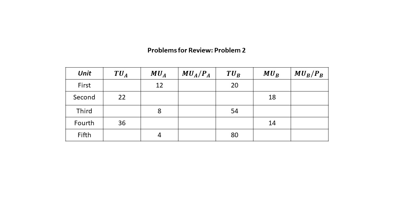
2. Assume that the price of good A is $1 per unit and the price of good B is $2 per unit. Complete the rest of the table.
3. Using the information from problem 2, assume that John has $14 of money income to spend on the two goods. How many units of each good will John purchase?
4. Suppose Bill has an income of $26 and faces constant prices for yogurt and pudding. Yogurt is $4 per pack and pudding is $5 per pack. Derive Bill’s budget equation and draw it on a graph. Label both axes and both intercepts. Place yogurt on the vertical axis.
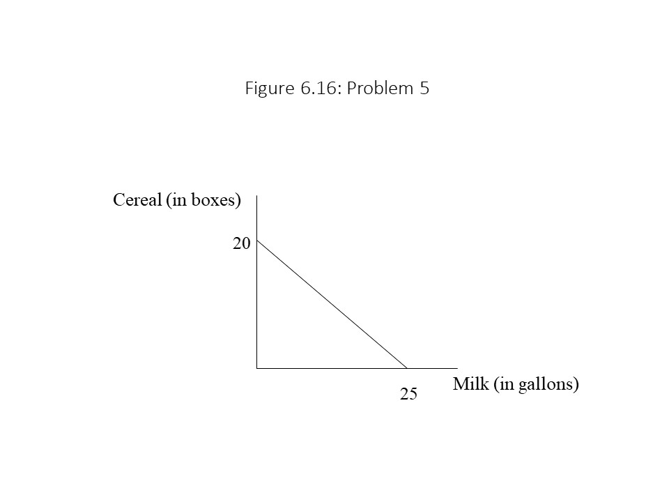
5. Consider the budget constraint shown in Figure 6.16. Suppose the price of cereal rises from $2.75 to $5.50 per box. What is the consumer’s income if the line represents the consumer’s initial budget line? Draw the new budget line on the same graph and label any new intercepts. Can you determine the price of milk (per gallon)?
6. Suppose the price of cigarettes (per pack) falls. How might the quantity purchased by a high school student be affected if her preferences are exogenously determined? How might her preferences be affected if her preferences are endogenously determined? Explain.
Samuelson and Nordhaus (2001), p. 85, encourage readers to “resist the idea that utility is a psychological function or feeling that can be observed or measured.” Instead, they regard it as a “scientific construct.” ↵
It is possible to construct an example in which a consumer has some money left over if that amount is not sufficient to pay the price of an additional unit of either good. ↵
The classical economists also recognized that the scarcity or abundance of a good would influence its price, but we can think of that characteristic as influencing the labor requirement. For example, if water is plentiful in a region, then the labor time required for its production will be lower. ↵
Neoclassical textbooks frequently discuss this paradox, but they typically do not acknowledge that the classical economists possessed an internally consistent solution to the paradox. I would like to acknowledge Prof. David Ruccio, whose lecture on this topic in an introductory economics class at the University of Notre Dame in the early 2000s influenced my presentation of this topic. I served as a teaching assistant for Prof. Ruccio at the time. ↵
The loss of utility for person A will probably be slightly more than 10 utils due to diminishing marginal utility. ↵
The reader should note that indifference curves with given preferences never cross. The only reason they appear to cross in this graph is because two different sets of indifference curves are being placed on the same graph. ↵


 These graphs of the TU and MU curves offer two different ways to visualize the law of diminishing marginal utility to which all individual consumers are subject, according to neoclassical economists. The law of diminishing marginal utility states that marginal utility declines as a consumer consumes more of a good. This reduction in MU is the result of the consumer attempting to satiate herself due to her consumption of the good. The marginal utility of each additional unit consumed is smaller and smaller until eventually an additional unit makes a negative addition to the total utility.
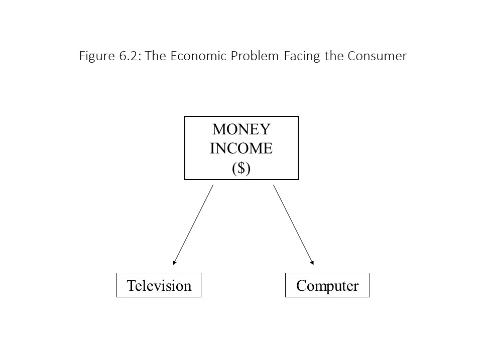 If the television will give the consumer 400 utils and the computer will give the consumer 800 utils, then one might conclude that the consumer should purchase the computer to maximize total utility. The problem with this line of reasoning is that it completely fails to consider the prices of the products. The price of the television might be $100 and the price of the computer might be $400. It turns out that the consumer will choose to purchase the television even though it gives the consumer less utility because the price is so much lower than the price of the computer.
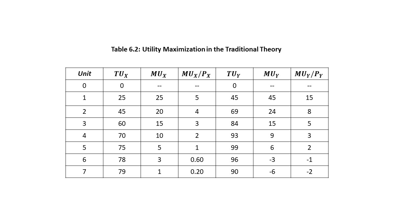
 Assume that the consumer is maximizing utility at the original price of PY. In other words, the initial condition when all income is spent is the following:
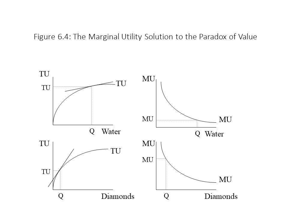 The top graphs in the figure show that the total utility obtained from the consumption of water is very high due to the large volume consumed. The marginal utility of the last unit consumed is very low for that same reason. The bottom graphs in the figure show that the total utility obtained from the consumption of diamonds is very low because of the small amount consumed. For the same reason, the marginal utility of the last diamond consumed is very high. The reader should also observe the straight lines that are just tangent to the TU curves at the quantities consumed. The slopes of the tangent lines represent the marginal utilities. The relatively flat tangent line in the top left graph indicates a low marginal utility. The relatively steep tangent line in the bottom left graph indicates a high marginal utility.
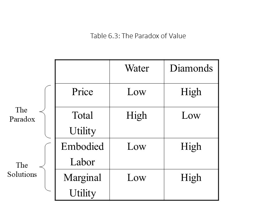 Criticisms of the Neoclassical Measure of Welfare
 Each point in the commodity space represents a commodity bundle, or a combination of the two goods. For example, the ordered pair (8, 6) represents a commodity bundle that includes 8 units of good X and 6 units of good Y.
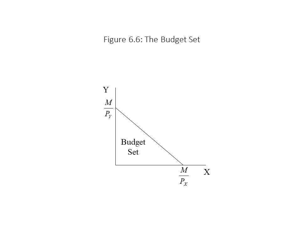 In economic terms, the vertical and horizontal intercepts refer to the maximum quantities of Y and X, respectively, that can be purchased if the consumer spends the entire money income on one or the other good. Each of the other points on the budget line represents a commodity bundle that requires the consumer to spend the entire money income. Bundles below the budget line are affordable but do not require the expenditure of the entire income. For example, if a consumer began at a bundle on the budget line and reduced the amount of Y by a small amount, then some income would be left over. Hence, that bundle would be affordable but would not require the expenditure of the entire income. All the bundles on the budget line and those below the budget line are affordable and are therefore considered part of the consumer’s budget set. Any bundle above the budget line is not affordable because the consumer would need more income than she possesses to make that purchase.
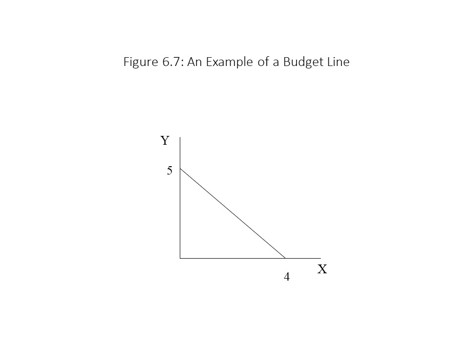 The reader should notice that the intercepts may be obtained quickly since M/PX = 4 and M/PY = 5. The slope may also be determined quickly because –PX/PY = –5/4 = –1.25. That is, if the consumer wishes to increase the consumption of X by one unit, then he must give up 1.25 units of Y.
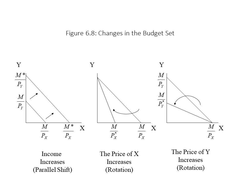
 All the bundles along indifference curve, U1, are equally preferred to all other bundles on that same indifference curve. It is also possible to identify regions that have more of both goods relative to bundle A, less of both goods relative to bundle A, more Y and less X relative to bundle A, and less Y and more X relative to bundle A.
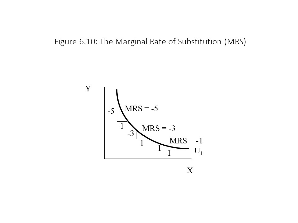 As the figure shows, when the MRS is – 5 (approximately) the consumer is willing to sacrifice 5 units of Y for one more unit of X. When the MRS is – 3 (approximately) the consumer is willing to sacrifice 3 units of Y for 1 more unit of X. Finally, when the MRS is – 1 the consumer is willing to sacrifice only 1 unit of Y for 1 more unit of X. Clearly, as the consumer consumes more X, the amount of Y he is willing to sacrifice to obtain another unit of X becomes smaller and smaller. In other words, X is becoming less valuable to the consumer as more of it is consumed. Although this result sounds a great deal like the law of diminishing marginal utility, it was obtained without the use of cardinal (quantifiable) utility. The only reason that we know the consumer values additional units of X less as more of it is consumed is that he is willing to give up less and less Y for those additional units. Diminishing marginal rate of substitution is the phrase we can use to refer to this tendency of the MRS to fall (in absolute value) as more X is consumed.
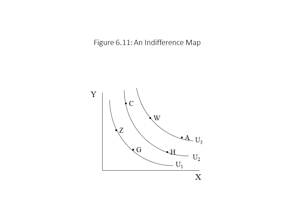 In the figure, a few commodity bundles have been labeled. Is it possible to identify the consumer’s ranking of these bundles? It is so long as we assume that more of both goods is always preferred to less of both goods. If we make this assumption, then it follows that any commodity bundle on a higher indifference curve must be preferred to any bundle on a lower indifference curve. In this case, W and A are equally preferred. W and A are strictly preferred to C and H, which are equally preferred to one another. Finally, Z and G are equally preferred to one another, and they are less preferred than C and H. We are free to state that W and A give the consumer the most utility, but since we are using an ordinal notion of utility, this statement only means that they are the most preferred bundles in the ranking.
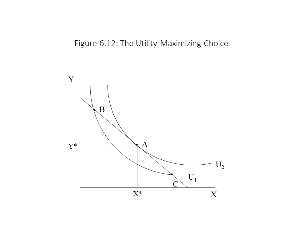 We want to determine what the utility maximizing commodity bundle is. We can begin by narrowing down the possibilities very quickly. The bundle that maximizes utility must be on the budget line. If it is not, then the consumer will have income left over. Because only the consumption of goods generates utility, the consumer cannot be maximizing utility unless she is consuming on the budget line.
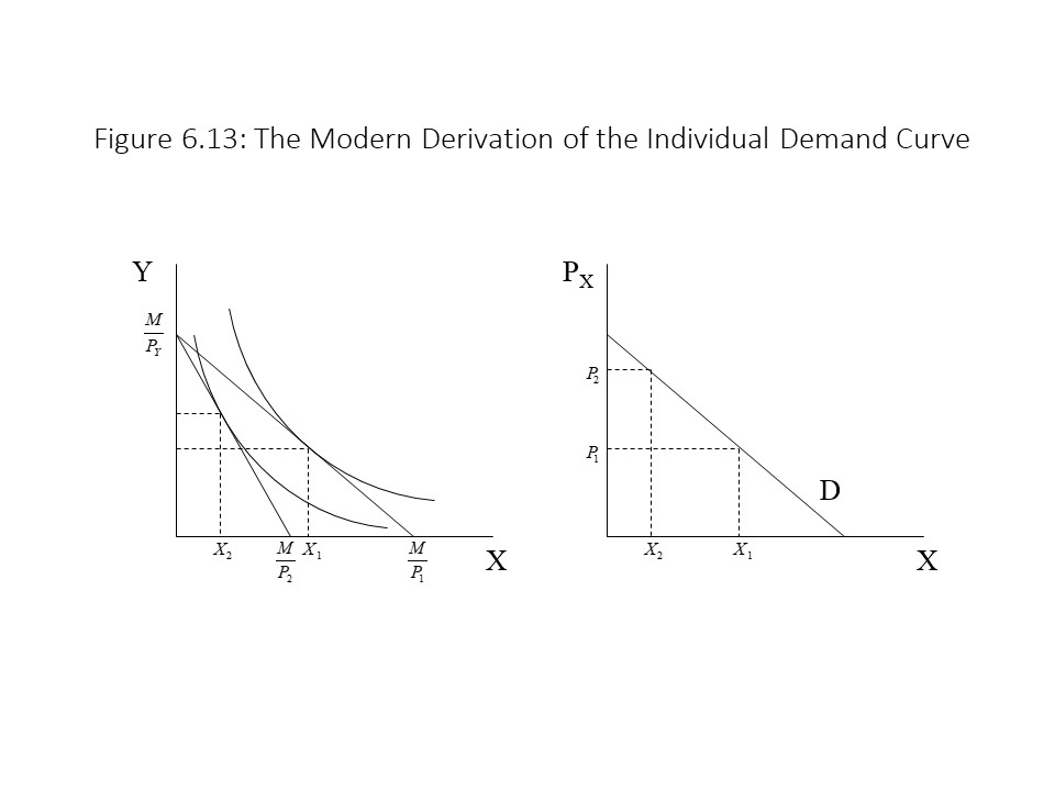 In Figure 6.13, the price of good X rises from P1 to P2, causing a rotation inward of the budget line. The consumer moves from one utility maximizing point to another. In this case, he reduces the quantity demanded of X from X1 units to X2 units. The result is a movement up the individual demand curve. Because the consumer moves to a lower indifference curve, it is apparent that the consumer’s level of satisfaction has diminished as he moves up the demand curve. This conclusion makes sense because the consumer now faces a higher price for good X and nothing else has changed about his situation. This analysis could easily be reversed with a decline in the price of good X and a rise in the quantity demanded of good X.
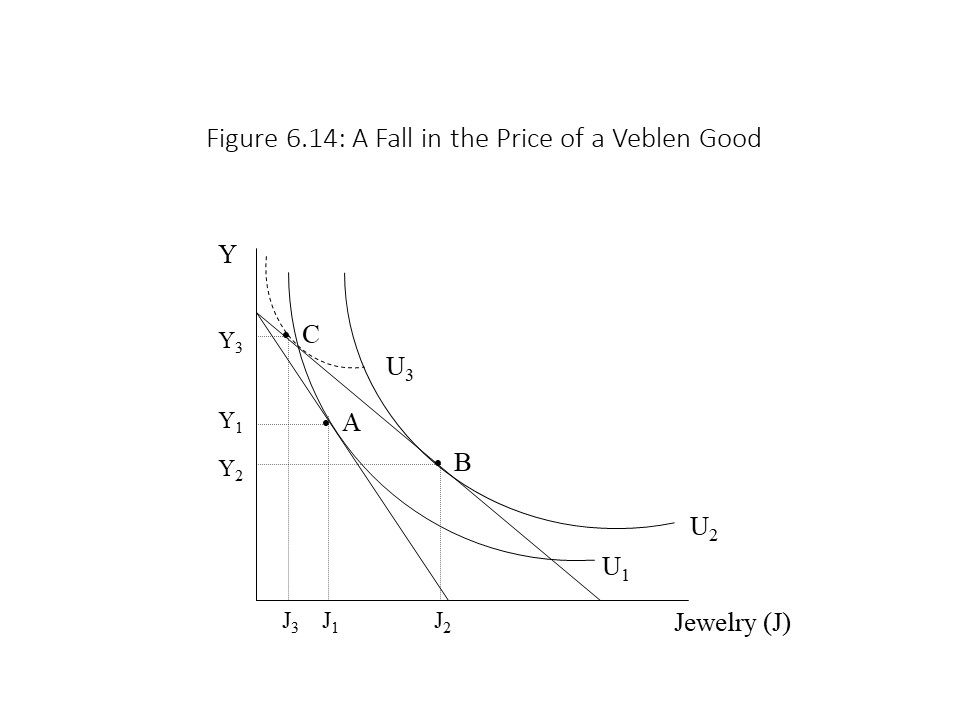 According to Figure 6.14, as the price of jewelry falls, the budget line rotates outward as usual. If preferences are given, then the quantity of jewelry that the consumer chooses increases from J1 to J2, and the consumer’s utility level rises from U1 to U2. In this case, however, preferences are endogenously determined. Because the price of jewelry has fallen, this wealthy consumer’s preferences change such that she prefers to purchase less jewelry rather than more. The indifference curves move such that the utility maximizing choice of jewelry is J3 at the lower price, and the utility level is U3.[7] Of course, less wealthy consumers might not experience any change in preferences when the price of jewelry falls, and they will purchase more.
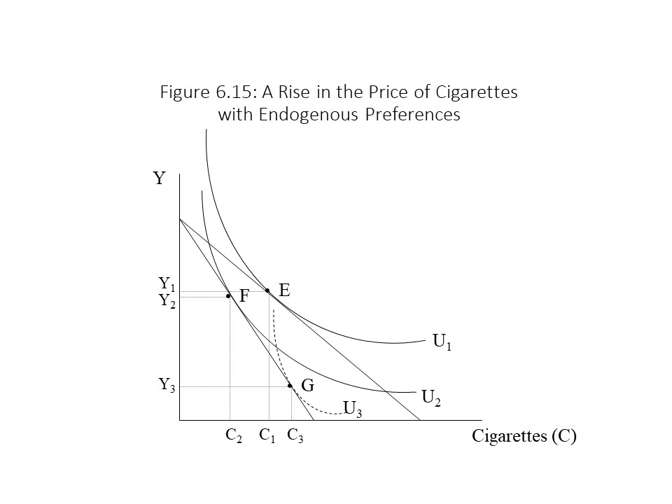 If preferences are exogenously determined, then the student will reduce his consumption of cigarettes from C1 to C2 and his utility will decline from U1 to U2. If preferences are endogenously determined, on the other hand, then it is possible that the rise in price will lead to greater profits for the tobacco companies. This increase in profits may be used to more aggressively advertise tobacco products to young people. The advertising campaign might change the preferences of the student so much that the student ends up purchasing more cigarettes even though the price rose. In Figure 6.15, the indifference curves move such that the final consumption of cigarettes is C3 and the student’s utility level is U3.