3.2: Monopoly Profit-Maximizing Solution

The profit-maximizing solution for the monopolist is found by locating the biggest difference between total revenues \((TR)\) and total costs \((TC)\), as in Equation \ref{3.1}.

\[\max π = TR – TC \label{3.1}\]

Monopoly Revenues

Revenues are the money that a firm receives from the sale of a product.

Total Revenue [TR] = The amount of money received when the producer sells the product. \(TR = PQ\)

Average Revenue [AR] = The average dollar amount receive per unit of output sold \(AR = \dfrac{TR}{Q}\)

Marginal Revenue [MR] = the addition to total revenue from selling one more unit of output.

\[\begin{align*} MR &= \frac{ΔTR}{ΔQ} = \frac{∂TR}{∂Q}.\\[4pt] TR &= PQ \text{ (USD)}\\[4pt] AR &= \frac{TR}{Q} = P\text{ (USD/unit)}\\[4pt] MR &= \frac{ΔTR}{ΔQ} = \frac{∂TR}{∂Q} \text{ (USD/unit)} \end{align*}\]

For the agricultural chemical company:

\[\begin{align*} TR &= PQ = (100 – Q)Q = 100Q – Q^2 \\[4pt] AR &= P = 100 – Q\\[4pt] MR &= \frac{∂TR}{∂Q} = 100 – 2Q \end{align*}\]

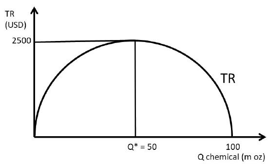
Total revenues for the monopolist are shown in Figure \(\PageIndex{1}\). Total Revenues are in the shape of an inverted parabola. The maximum value can be found by taking the first derivative of TR, and setting it equal to zero. The first derivative of TR is the slope of the TR function, and when it is equal to zero, the slope is equal to zero.

\[\max TR = PQ \frac{∂TR}{∂Q} = 100 – 2Q = 0 Q^* = 50 \label{3.2}\]

Substitution of \(Q^*\) back into the \(TR\) function yields \(TR = \text{ USD } 2500\), the maximum level of total revenues (Figure \(\PageIndex{1}\)).

Figure \(\PageIndex{1}\): Total Revenues for a Monopolist: Agricultural Chemical

Figure \(\PageIndex{2}\): Per-Unit Revenues for a Monopolist: Agricultural Chemical

It is important to point out that the optimal level of chemical is not this level. The optimal level of chemical to produce and sell is the profit-maximizing level, which is revenues minus costs. If the monopolist were to maximize revenues instead of profits, it might cost too much relative to the gain in revenue. Profits include both revenues and costs.

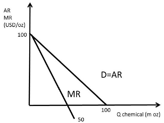
Average revenue \((AR)\) and marginal revenue \((MR)\) are shown in Figure \(\PageIndex{2}\). The marginal revenue curve has the same y-intercept and twice the slope as the average revenue curve. This is always true for linear demand (average revenue) curves. This is one of the major take home messages of economics: maximize revenues may cost too much to make it worth it. For example, a corn farmer who maximizes yield (output per acre of land) may be spending too much on inputs such as fertilizer and chemicals make the higher yield payoff. From an economic perspective, the corn farmer should consider both revenues and costs.

Monopoly Costs

The costs for the chemical include total, average, and marginal costs.

Total Cost [TC] = The sum of all payments that a firm must make to purchase the factors of production. The sum of Total Fixed Costs and Total Variable Costs. \(TC = C(Q) = TFC + TVC.\)

Total Fixed Costs [TFC] = Costs that do not vary with the level of output.

Total Variable Costs [TVC] = Costs that do vary with the level of output.

Average Cost [AC] = total costs per unit of output. \(AC = \dfrac{TC}{Q}\). Note that the terms, Average Costs and Average Total Costs are interchangeable.

Marginal Cost [MC] = the increase in total costs due to the production of one more unit of output. \(MC = \dfrac{ΔTC}{ΔQ} = \dfrac{∂TC}{∂Q}\).

\[\begin{align*} TC &= C(Q)\text{ (USD)}\\[4pt] AC &= \frac{TC}{Q}\text{ (USD/unit)}\\[4pt] MC &= \frac{ΔTC}{ΔQ} = \frac{∂TC}{∂Q} \text{ (USD/unit)}\end{align*}\]

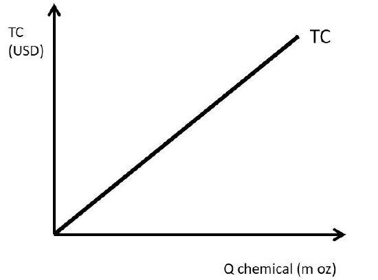
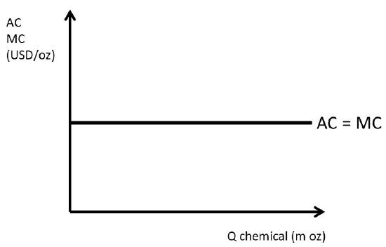
Suppose that the agricultural chemical firm is a constant cost industry. This means that the per-unit cost of producing one more ounce of chemical is the same, no matter what quantity is produced. Assume that the cost per unit is ten dollars per ounce (10 USD/oz).

\[\begin{align*} TC &= 10Q\\[4pt] AC &= \frac{TC}{Q} = 10\\[4pt] MC &= \frac{ΔTC}{ΔQ} = \frac{∂TC}{∂Q} = 10\end{align*}\]

The total costs are shown in Figure \(\PageIndex{3}\), and the per-unit costs are in Figure \(\PageIndex{4}\).

Figure \(\PageIndex{3}\): Total Costs for a Monopolist: Agricultural Chemical

Figure \(\PageIndex{4}\): Per-Unit Costs for a Monopolist: Agricultural Chemical

Monopoly Profit-Maximizing Solution

There are three ways to communicate economics: verbally, graphically, and mathematically. The firm’s profit maximizing solution is one of the major features and important conclusions of economics. The verbal explanation is that a firm should continue any activity as long as the additional (marginal) benefits are greater than the additional (marginal) costs. The firm should continue the activity until the marginal benefit is equal to the marginal cost. This is true for any activity, and for profit maximization, the firm will find the optimal, profit maximizing level of output where marginal revenues equal marginal costs \((MR = MC)\).

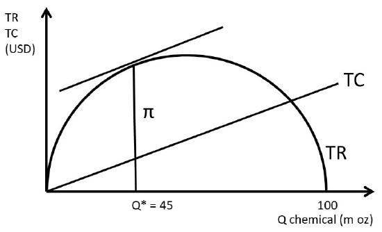
The graphical solution takes advantage of pictures that tell the same story, as in Figures \(\PageIndex{5}\) and \(\PageIndex{6}\). Figure \(\PageIndex{5}\) shows the profit maximizing solution using total revenues and total costs. The profit-maximizing level of output is found where the distance between \(TR\) and \(TC\) is largest: \(π = TR – TC\). The solution is found by setting the slope of \(TR\) equal to the slope of \(TC\): this is where the rates of change are equal to each other \((MR = MC)\).

Figure \(\PageIndex{5}\): Total Profit Solution for a Monopolist: Agricultural Chemical

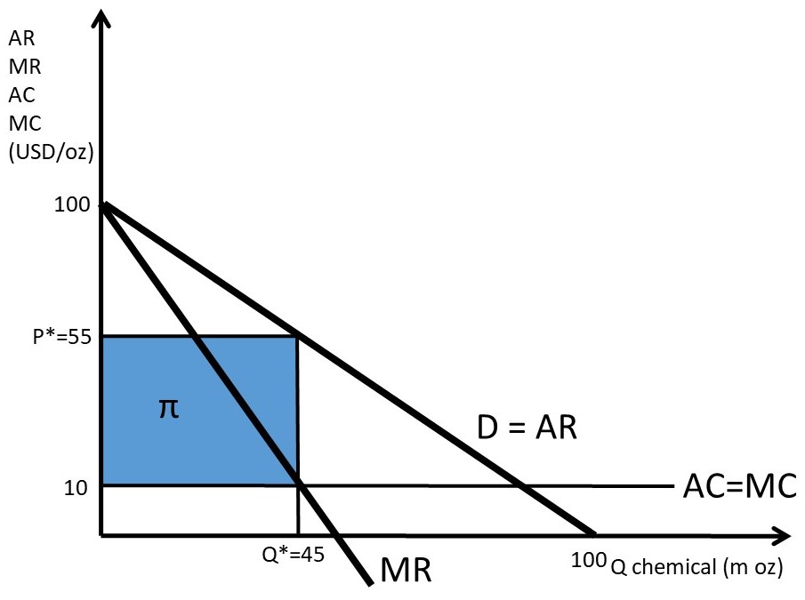
The same solution can be found using the marginal graph (Figure \(\PageIndex{6}\)). The firm sets \(MR\) equal to \(MC\) to find the profit-maximizing level of output \((Q^*)\), then substitutes \(Q^*\) into the consumers’ willingness to pay (demand curve) to find the optimal price \((P^*)\). The profit level is an area in Figure \(\PageIndex{6}\), defined by \(TR\) and \(TC\). Total revenues are equal to price times quantity \((TR = P^*Q)\), so \(TR\) are equal to the rectangle from the origin to \(P^*\) and \(Q^*\). Total costs are equal to the rectangle defined by the per-unit cost of ten dollars per ounce times the quantity produced, \(Q^*\). If the \(TC\) rectangle is subtracted from the TR rectangle, the shaded profit rectangle remains: profits are the residual of revenues after all costs have been paid \((π = TR – TC)\).

Figure \(\PageIndex{6}\): Marginal Profit Solution for a Monopolist: Agricultural Chemical

The math solution for profit maximization is found by using calculus. The maximum level of a function is found by taking the first derivative and setting it equal to zero. Recall that the inverse demand function facing the monopolist is \(P = 100 – Q^d\), and the per unit costs are ten dollars per ounce.

\[\begin{align*} \max π &= TR – TC\\[4pt] &= P(Q)Q – C(Q)\\[4pt] &= (100 – Q)Q – 10Q\\[4pt] &= 100Q – Q^2 – 10Q\\[4pt] \frac{∂π}{∂Q} &= 100 – 2Q – 10 = 0\\[4pt] 2Q &= 90\\[4pt] Q^* &= 45 \text{ million ounces of agricultural chemical}\end{align*}\]

The profit-maximizing price is found by substituting \(Q^*\) into the inverse demand equation:

\[P^* = 100 – Q^* = 100 – 45 = 55 \text{ USD/ounce of agricultural chemical}.\nonumber\]

The maximum profit level can be found by substitution of \(P^*\) and \(Q^*\) into the profit equation:

\[π = TR – TC = P(Q)Q – C(Q) = 55\cdot 45 – 10\cdot 45 = 45\cdot 45 = 2025 \text{ million USD}.\nonumber\]

This profit level is equal to the distance between the \(TR\) and \(TC\) curves at \(Q^*\) in Figure \(\PageIndex{5}\), and the profit rectangle identified in Figure \(\PageIndex{6}\). The profit-maximizing level of output and price have been found in three ways: verbally, graphically, and mathematically.