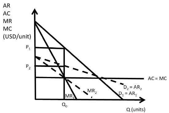
There is no supply curve for a monopolist. This differs from a competitive industry, where there is a one-to-one correspondence between price \((P)\) and quantity supplied \((Q^s)\). For a monopoly, the price depends on the shape of the demand curve, as shown in Figure \(\PageIndex{1}\). A mathematical “function” is defined as a one-to-one correspondence between each point in the range \((x)\) and the domain \((y)\). A supply curve, then, requires a single price \((P)\) for each quantity \((Q)\). This graph shows that there is more than one price associated with each quantity. At quantity \(Q_0\), for demand curve \(D_1\), the monopolist maximizes profits by setting \(MR_1 = MC\), which results in price \(P_1\). However, for demand curve \(D_2\), the monopolist would set \(MR_2=MC\), and charge a lower price, \(P_2\). Since there is more than one price associated with a single quantity \((Q_0)\), there is no one-to-one correspondence between price and quantity supplied, and no supply curve for a monopolist.
Figure \(\PageIndex{1}\): Absence of a Supply Curve for a Monopolist
The Effect of a Tax on a Monopolist’s Price
In a competitive industry, a tax results in an increase in price that is based on the incidence of the tax. The price increase is a fraction of the tax, less than the tax amount. The tax incidence depends on the magnitude of the elasticities of supply and demand. In a monopoly, it is possible that the price increase from a tax is greater than the tax itself, as shown in Figure \(\PageIndex{2}\). This is an interesting and nonintuitive result!
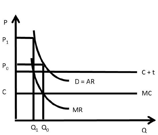
Before the tax, the monopolist sets \(MR = MC\) at \(Q_0\), and sets price at \(P_0\). After the tax is imposed, the marginal costs increase to \(C + t\). The monopolist sets \(MR = MC = C + t\), produces quantity \(Q_1\), and charges price \(P_1\). The increase in price \((P_1 – P_0)\) is larger than the tax rate \((t)\), the vertical distance between the \(C + t\) and \(MC\) lines. In this case, consumers of the monopoly good are paying more than 100 percent of the tax rate. This is because of the shape of the demand curve: it is profitable for the monopoly to reduce quantity produced to increase the price.
Figure \(\PageIndex{2}\): The Effect of a Tax on a Monopolist’s Price
Multiplant Monopolist
Suppose that a monopoly has two or more plants (factories). How does the monopolist determine how much output should be produced at each plant? Profit-maximization suggests two guidelines for the multiplant monopolist. Suppose that the monopolist operates \(n\) plants.
Set \(MC\) equal across all plants: \(MC_1 = MC_2 = … = MC_n\), and
Set \(MR = MC\) in all plants.
A mathematical model of a multiplant monopolist demonstrates profit-maximization. The result is interesting and important, as it shows that multiplant firms will not always close older, less efficient plants. This is true even if the older plants have higher production costs than newer, more efficient plants.
Suppose that a monopolist has two plants, and total output \((Q_T)\) is the sum of output produced in plant 1 \((Q_1)\) and plant 2 \((Q_2)\).
\[Q_1 + Q_2 = Q_T \label{3.6}\]
The profit-maximizing model for the two-plant monopolist yields the solution. The costs of producing output in each plant differ. Assume that the old plant (plant 1) is less efficient than the new plant (plant 2): \(C_1 > C_2\).
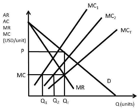
The multiplant monopolist solution is shown in Figure \(\PageIndex{3}\). The marginal cost curve for plant 1 is higher than the marginal cost curve for plant 2, reflecting the older, less efficient plant. Rather than shutting the less efficient plant down, the monopolist should produce some output in each plant, and set the \(MC\) of each plant equal to \(MR\), as shown in the graph. Let \(MC_T\) be the total (sum) of the marginal cost curves: \(M_T = MC_1 + MC_2\). The profit maximizing quantity \((Q_T)\) is found by setting \(MR\) equal to \(MC_T\). At the profit maximizing quantity \((Q_T)\), the monopolist sets price equal to \(P\), found by plugging \(Q_T\) into the consumers’ willingness to pay, or the demand curve \((D)\).
Figure \(\PageIndex{3}\): Multiplant Monopolist
To find the quantity to produce in each plant, the firm sets \(MC_1 = MC_2 = MC_T\) to find the profit-maximizing level of output in each plant: \(Q_1\) and \(Q_2\). The outcome of the multiplant monopolist yields useful conclusions for any firm: continue using any input, plant, or resource until marginal costs equal marginal revenues. Less efficient resources can be usefully employed, even if more efficient resources are available. The next section will explore the determinants and measurement of monopoly power, also called market power.