
5.3: Oligopoly Models
- Last updated
- Save as PDF
- Page ID
- 43177

An oligopoly is defined as a market structure with few firms and barriers to entry.
Oligopoly = A market structure with few firms and barriers to entry.
There is often a high level of competition between firms, as each firm makes decisions on prices, quantities, and advertising to maximize profits. Since there are a small number of firms in an oligopoly, each firm’s profit level depends not only on the firm’s own decisions, but also on the decisions of the other firms in the oligopolistic industry.
Strategic Interactions
Each firm must consider both: (1) other firms’ reactions to a firm’s own decisions, and (2) the own firm’s reactions to the other firms’ decisions. Thus, there is a continuous interplay between decisions and reactions to those decisions by all firms in the industry. Each oligopolist must take into account these strategic interactions when making decisions. Since all firms in an oligopoly have outcomes that depend on the other firms, these strategic interactions are the foundation of the study and understanding of oligopoly.
For example, each automobile firm’s market share depends on the prices and quantities of all of the other firms in the industry. If Ford lowers prices relative to other car manufacturers, it will increase its market share at the expense of the other automobile companies.
When making decisions that consider the possible reactions of other firms, firm managers usually assume that the managers of competing firms are rational and intelligent. These strategic interactions form the study of game theory, the topic of Chapter 6 below. John Nash (1928-2015), an American mathematician, was a pioneer in game theory. Economists and mathematicians use the concept of a Nash Equilibrium \((NE)\) to describe a common outcome in game theory that is frequently used in the study of oligopoly.
Nash Equilibrium = An outcome where there is no tendency to change based on each individual choosing a strategy given the strategy of rivals.
In the study of oligopoly, the Nash Equilibrium assumes that each firm makes rational profit-maximizing decisions while holding the behavior of rival firms constant. This assumption is made to simplify oligopoly models, given the potential for enormous complexity of strategic interactions between firms. As an aside, this assumption is one of the interesting themes of the motion picture, “A Beautiful Mind,” starring Russell Crowe as John Nash. The concept of Nash Equilibrium is also the foundation of the models of oligopoly presented in the next three sections: the Cournot, Bertrand, and Stackelberg models of oligopoly.
Cournot Model
Augustin Cournot (1801-1877), a French mathematician, developed the first model of oligopoly explored here. The Cournot model is a model of oligopoly in which firms produce a homogeneous good, assuming that the competitor’s output is fixed when deciding how much to produce.
A numerical example of the Cournot model follows, where it is assumed that there are two identical firms (a duopoly), with output given by \(Q_i (i=1,2)\). Therefore, total industry output is equal to: \(Q = Q_1 + Q_2\). Market demand is a function of price and given by \(Q^d = Q^d(P)\), thus the inverse demand function is \(P = P(Q^d)\). Note that the price depends on the market output \(Q\), which is the sum of both individual firm’s outputs. In this way, each firm’s output has an influence on the price and profits of both firms. This is the basis for strategic interaction in the Cournot model: if one firm increases output, it lowers the price facing both firms. The inverse demand function and cost function are given in Equation \ref{5.1}.
\[P = 40 – QC(Q_i) = 7Q_i \label{5.1}\]
with \(i = 1,2\).
Each firm chooses the optimal, profit-maximizing output level given the other firm’s output. This will result in a Nash Equilibrium, since each firm is holding the behavior of the rival constant. Firm One maximizes profits as follows.
\[\begin{align*} \max π_1 &= TR_1 – TC_1\\[4pt] \max π_1 &= P(Q)Q_1 – C(Q_1) \text{ [price depends on total output } Q = Q_1 + Q_2]\\[4pt] \max π_1 &= [40 – Q]Q_1 – 7Q_1\\[4pt] \max π_1 &= [40 – Q_1 – Q_2]Q_1 – 7Q_1\\[4pt] \max π_1 &= 40Q_1 – Q_1^2 – Q_2Q_1 – 7Q_1\\[4pt] \frac{∂π_1}{∂Q_1} &= 40 – 2Q_1 – Q_2 – 7 = 0\\[4pt] 2Q_1 &= 33 – Q_2\\[4pt] Q_1^* &= 16.5 – 0.5Q_2\end{align*}\]
This equation is called the “Reaction Function” of Firm One. This is as far as the mathematical solution can be simplified, and represents the Cournot solution for Firm One. It is a reaction function since it describes Firm One’s reaction given the output level of Firm Two. This equation represents the strategic interactions between the two firms, as changes in Firm Two’s output level will result in changes in Firm One’s response. Firm One’s optimal output level depends on Firm Two’s behavior and decision making. Oligopolists are interconnected in both behavior and outcomes.
The two firms are assumed to be identical in this duopoly. Therefore, Firm Two’s reaction function will be symmetrical to the Firm One’s reaction function (check this by setting up and solving the profit-maximization equation for Firm Two):
\[Q_2^* = 16.5 – 0.5Q_1\nonumber\]
The two reaction functions can be used to solve for the Cournot-Nash Equilibrium. There are two equations and two unknowns \((Q_1\) and \(Q_2)\), so a numerical solution is found through substitution of one equation into the other.
\[\begin{align*} Q_1^* &= 16.5 – 0.5(16.5 – 0.5Q_1)\\[4pt] Q_1^* &= 16.5 – 8.25 + 0.25Q_1\\[4pt] Q_1^* &= 8.25 + 0.25Q_1\\[4pt] 0.75Q_1^* &= 8.25\\[4pt] Q_1^* &= 11\end{align*}\]
Due to symmetry from the assumption of identical firms:
\[\begin{align*} Q_i &= 11 & i &= 1,2\\[4pt] Q &= 22\text{ units}\\[4pt]P &= 18 \text{ USD/unit}\end{align*}\]
Profits for each firm are:
\[π_i = P(Q)Q_i – C(Q_i) = 18(11) – 7(11) = (18 – 7)11 = 11(11) = 121 \text{ USD}\nonumber\]
This is the Cournot-Nash solution for oligopoly, found by each firm assuming that the other firm holds its output level constant. The Cournot model can be easily extended to more than two firms, but the math does get increasingly complex as more firms are added. Economists utilize the Cournot model because is based on intuitive and realistic assumptions, and the Cournot solution is intermediary between the outcomes of the two extreme market structures of perfect competition and monopoly.
This can be seen by solving the numerical example for competition, Cournot, and monopoly models, and comparing the solutions for each market structure.
In a competitive industry, free entry results in price equal to marginal cost \((P = MC)\). In the case of the numerical example, \(P_C = 7\). When this competitive price is substituted into the inverse demand equation, \(7 = 40 – Q\), or \(Q_c = 33\). Profits are found by solving \((P – MC)Q\), or \(π_c = (7 – 7)Q = 0\). The competitive solution is given in Equation \ref{5.2}.
\[P_c = 7 \text{ USD/unit } Q_c = 33 \text{ units } π_c = 0 \text{ USD}\label{5.2}\]
The monopoly solution is found by maximizing profits as a single firm.
\[\begin{align*} \max π_m &= TR_m – TC_m\\[4pt] \max π_m &= P(Q_m)Q_m – C(Q_m)\text{ [price depends on total output } Q_m]\\[4pt] \max π_m &= [40 – Q_m]Q_m – 7Q_m\\[4pt] \max π_m &= 40Q_m – Q_m^2 – 7Q_m\end{align*}\]
\[\begin{align*} \frac{∂π_m}{∂Q_m} &= 40 – 2Q_m – 7 = 0\\[4pt] 2Q_m &= 33\\[4pt] Q_m^* &= 16.5\\[4pt] P_m &= 40 – 16.5 = 23.5\\[4pt]π_m &= (P_m – MC_m)Q_m = (23.5 – 7)16.5 = 16.5(16.5) = 272.25 \text{ USD}\end{align*}\]
The monopoly solution is given in Equation \ref{5.3}.
\[\begin{align} P_m &= 23.5 \text{ USD/unit} \label{5.3} \\[4pt] Q_m &= 16.5 \text{ units}\nonumber \\[4pt] π_m &= 272.5 \text{ USD}\nonumber \end{align}\]
The competitive, Cournot, and monopoly solutions can be compared on the same graph for the numerical example (Figure \(\PageIndex{1}\)).
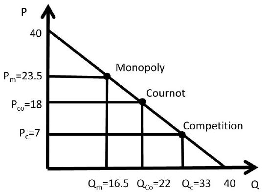
The Cournot price and quantity are between perfect competition and monopoly, which is an expected result, since the number of firms in an oligopoly lies between the two market structure extremes.
Bertrand Model
Joseph Louis François Bertrand (1822-1900) was also a French mathematician who developed a competing model to the Cournot model. Bertrand asked the question, “what would happen in an oligopoly model if each firm held the other firm’s price constant?” The Bertrand model is a model of oligopoly in which firms produce a homogeneous good, and each firm takes the price of competitors fixed when deciding what price to charge.
Assume two firms in an oligopoly (a duopoly), where the two firms choose the price of their good simultaneously at the beginning of each period. Consumers purchase from the firm with the lowest price, since the products are homogeneous (perfect substitutes). If the two firms charge the same price, one-half of the consumers buy from each firm. Let the demand equation be given by \(Q^d = Q^d(P)\). The Bertrand model follows these three statements:
- If \(P_1 < P_2\), then Firm One sells \(Q^d\) and Firm Two sells 0,
- If \(P_1 > P_2\), then Firm One sells 0 and Firm Two sells \(Q^d\), and
- If \(P_1 = P_2\), then Firm One sells \(0.5Q^d\) and Firm Two sells \(0.5Q^d\).
A numerical example demonstrates the outcome of the Bertrand model, which is a Nash Equilibrium. Assume two firms sell a homogeneous product, and compete by choosing prices simultaneously, while holding the other firm’s price constant. Let the demand function be given by \(Q^d = 50 – P\) and the costs are summarized by \(MC_1 = MC_2 = 5\).
(1) Firm One sets \(P_1 = 20\), and Firm Two sets \(P_2 = 15\). Firm Two has the lower price, so all customers purchase the good from Firm Two.
\[\begin{align*} Q_1 &= 0\\[4pt] Q_2 &= 35\\[4pt] π_1 &= 0\\[4pt] π_2 &= (15 – 5)35 = 350 \text{ USD}.\end{align*}\]
After period one, Firm One has a strong incentive to lower the price \((P_1)\) below \(P_2\).The Bertrand assumption is that both firms will choose a price, holding the other firm’s price constant. Thus, Firm One undercuts \(P_2\) slightly, assuming that Firm Two will maintain its price at \(P_2 = 15\). Firm Two will keep the same price, assuming that Firm One will maintain \(P_1 = 20\).
(2) Firm One sets \(P_1 = 14\), and Firm Two sets \(P_2 = 15\). Firm One has the lower price, so all customers purchase the good from Firm One.
\[\begin{align*} Q_1 &= 36\\[4pt] Q_2 &= 0\\[4pt] π_1&= (14 – 5)36 = 324 \text{ USD},\\[4pt] π_2 &= 0.\end{align*}\]
After period two, Firm Two has a strong incentive to lower price below \(P_1\). This process of undercutting the other firm’s price will continue and a “price war” will result in the price being driven down to marginal cost. In equilibrium, both firms lower their price until price is equal to marginal cost: \(P_1 = P_2 = MC_1 = MC_2\). The price cannot go lower than this, or the firms would go out of business due to negative economic profits. To restate the Bertrand model, each firm selects a price, given the other firm’s price. The Bertrand results are given in Equation \ref{5.4}.
\[\begin{align} P_1 &= P_2 = MC_1 = MC_2 \label{5.4} \\[4pt] Q_1 &= Q_2 = 0.5Q_d\nonumber \\[4pt] π_1 &= π_2 = 0 \text{ in the } SR \text{ and } LR.\nonumber \end{align}\]
The Bertrand model of oligopoly suggests that oligopolies are characterized by the competitive solution, due to competing over price. There are many oligopolies that behave this way, such as gasoline stations at a given location. Other oligopolies may behave more like Cournot oligopolists, with an outcome somewhere in between perfect competition and monopoly.
Stackelberg Model
Heinrich Freiherr von Stackelberg (1905-1946) was a German economist who contributed to game theory and the study of market structures with a model of firm leadership, or the Stackelberg model of oligopoly. This model assumes that there are two firms in the industry, but they are asymmetrical: there is a “leader” and a “follower.” Stackelberg used this model of oligopoly to determine if there was an advantage to going first, or a “first-mover advantage.”
A numerical example is used to explore the Stackelberg model. Assume two firms, where Firm One is the leader and produces \(Q_1\) units of a homogeneous good. Firm Two is the follower, and produces \(Q_2\) units of the good. The inverse demand function is given by \(P = 100 – Q\), where \(Q = Q_1 + Q_2\). The costs of production are given by the cost function: \(C(Q) = 10Q\).
This model is solved recursively, or backwards. Mathematically, the problem must be solved this way to find a solution. Intuitively, each firm will hold the other firm’s output constant, similar to Cournot, but the leader must know the follower’s best strategy to move first. Thus, Firm One solves Firm Two’s profit maximization problem to know what output it will produce, or Firm Two’s reaction function. Once the reaction function of the follower (Firm Two) is known, then the leader (Firm One) maximizes profits by substitution of Firm Two’s reaction function into Firm One’s profit maximization equation. All of this is shown in the following example.
Firm One starts by solving for Firm Two’s reaction function:
\[\begin{align*} \max π_2 &= TR_2 – TC_2\\[4pt]\max π_2 &= P(Q)Q_2 – C(Q_2)& &\text{[price depends on total output } Q = Q_1 + Q_2]\\[4pt] \max π_2 &= [100 – Q]Q_2 – 10Q_2\\[4pt] \max π_2 &= [100 – Q_1 – Q_2]Q_2 – 10Q_2\\[4pt] \max π_2 &= 100Q_2 – Q_1Q_2 – Q_2^2 – 10Q_2\\[4pt] \frac{∂π_2}{∂Q_2} &= 100 – Q_1 – 2Q_2 – 10 = 0\\[4pt] 2Q_2 &= 90 – Q_1\\[4pt] Q_2^* &= 45 – 0.5Q_1\end{align*}\]
This is the reaction function of the follower, Firm Two. Next, Firm One, the leader, maximizes profits holding the follower’s output constant using the reaction function.
\[\begin{align*} \max π_1 &= TR_1 – TC_1\\[4pt] \max π_1 &= P(Q)Q_1 – C(Q_1)& &\text{[price depends on total output } Q = Q1 + Q2] \\[4pt] \max π_1 &= [100 – Q]Q_1 – 10Q_1\\[4pt] \max π_1 &= [100 – Q_1 – Q_2]Q_1 – 10Q_1\\[4pt] \max π_1 &= [100 – Q1 – (45 – 0.5Q_1)]Q_1 – 10Q_1 & &\text{[substitution of One’s reaction function]}\\[4pt] \max π_1 &= [100 – Q_1 – 45 + 0.5Q_1]Q_1 – 10Q_1\\[4pt] \max π_1 &= [55 – 0.5Q_1]Q_1 – 10Q_1\\[4pt] \max π_1 &= 55Q_1 – 0.5Q_1^2 – 10Q_1\\[4pt] \frac{∂π_1}{∂Q_1} &= 55 – Q_1 – 10 = 0\\[4pt] Q_1^* &= 45\end{align*}\]
This can be substituted back into Firm Two’s reaction function to solve for \(Q_2^*\).
\[\begin{align*} Q_2^* &= 45 – 0.5Q_1 = 45 – 0.5(45) = 45 – 22.5 = 22.5\\[4pt] Q &= Q_1 + Q_2 = 45 + 22.5 = 67.5\\[4pt] P &= 100 – Q = 100 – 67.5 = 32.5\\[4pt] π_1 &= (32.5 – 10)45 = 22.5(45) = 1012.5 \text{ USD}\\[4pt] π_2 &= (32.5 – 10)22.5 = 22.5(22.5) = 506.25 \text{ USD}\end{align*}\]
We have now covered three models of oligopoly: Cournot, Bertrand, and Stackelberg. These three models are alternative representations of oligopolistic behavior. The Bertand model is relatively easy to identify in the real world, since it results in a price war and competitive prices. It may be more difficult to identify which of the quantity models to use to analyze a real-world industry: Cournot or Stackelberg?
The model that is most appropriate depends on the industry under investigation.
- The Cournot model may be most appropriate for an industry with similar firms, with no market advantages or leadership.
- The Stackelberg model may be most appropriate for an industry dominated by relatively large firms.
Oligopoly has many different possible outcomes, and several economic models to better understand the diversity of industries. Notice that if the firms in an oligopoly colluded, or acted as a single firm, they could achieve the monopoly outcome. If firms banded together to make united decisions, the firms could set the price or quantity as a monopolist would. This is illegal in many nations, including the United States, since the outcome is anti-competitive, and consumers would have to pay monopoly prices under collusion.
If firms were able to collude, they could divide the market into shares and jointly produce the monopoly quantity by restricting output. This would result in the monopoly price, and the firms would earn monopoly profits. However, under such circumstances, there is always an incentive to “cheat” on the agreement by producing and selling more output. If the other firms in the industry restricted output, a firm could increase profits by increasing output, at the expense of the other firms in the collusive agreement. We will discuss this possibility in the next section.
To summarize our discussion of oligopoly thus far, we have two models that assume that a firm holds the other firm’s output constant: Cournot and Stackelberg. These two models result in positive economic profits, at a level between perfect competition and monopoly. The third model, Bertrand, assumes that each firm holds the other firm’s price constant. The Bertrand model results in zero economic profits, as the price is bid down to the competitive level, \(P = MC\).
The most important characteristic of oligopoly is that firm decisions are based on strategic interactions. Each firm’s behavior is strategic, and strategy depends on the other firms’ strategies. Therefore, oligopolists are locked into a relationship with rivals that differs markedly from perfect competition and monopoly.