8.2: Case studies

8.2.1 Collocational frameworks and grammar patterns

An early extension of collocation research to the association between words and grammatical structure is Renouf & Sinclair (1991). The authors introduce a novel construct, the collocational framework, which they define as “a discontinuous sequence of two words, positioned at one word remove from each other”, where the two words in question are always function words – examples are [a __ of ], [an __ of ], [too __ to] or [many __ of ] (note that a and an are treated as constituents of different collocational frameworks, indicating a radically word-form-oriented approach to grammar). Renouf and Sinclair are particularly interested in classes of items that fill the position in the middle of collocational frameworks and they see the fact that these items tend to form semantically coherent classes as evidence that collocational frameworks are relevant items of linguistic structure.

The idea behind collocational frameworks was subsequently extended by Hunston & Francis (2000) to more canonical linguistic structures, ranging from very general valency patterns (such as [V NP] or [V NP NP]) to very specific structures like [there + Linking Verb + something Adjective + about NP] (as in There was something masculine about the dark wood dining room (Hunston & Francis 2000: 51, 53, 106)). Their essential insight is similar to Renouf and Sinclair’s: that such structures (which they call “grammar patterns”) are meaningful and that their meaning manifests itself in the collocates of their central slots:

The patterns of a word can be defined as all the words and structures which are regularly associated with the word and which contribute to its meaning. A pattern can be identified if a combination of words occurs relatively frequently, if it is dependent on a particular word choice, and if there is a clear meaning associated with it (Hunston & Francis 2000: 37).

Collocational frameworks and especially grammar patterns have an immediate applied relevance: the COBUILD dictionaries included the most frequently found patterns for each word in their entries from 1995 onward, and there is a two-volume descriptive grammar of the patterns of verbs (Francis et al. 1996) and nouns and adjectives (Francis et al. 1998); there were also attempts to identify grammar patterns automatically (cf. Mason & Hunston 2004). Research on collocational frameworks and grammar patterns is mainly descriptive and takes place in applied contexts, but Hunston & Francis (2000) argue very explicitly for a usage-based theory of grammar on the basis of their descriptions (note that the definition quoted above is strongly reminiscent of the way constructions were later defined in construction grammar (Goldberg 1995: 4), a point I will return to in the Epilogue of this book).

8.2.1.1 Case study: [a __ of]

As an example of a collocational framework, consider [a __ of ], one of the patterns that Renouf & Sinclair (1991) use to introduce their construct. Renouf and Sinclair use an early version of the Birmingham Collection of English Text, which is no longer accessible. To enable us to look at the methodological issues raised by collocational frameworks more closely, I have therefore replicated their study using the BNC. As far as one can tell from the data presented in Renouf & Sinclair (1991), they simply extracted all words occurring in the framework, without paying attention to part-of-speech tagging, so I did the same; it is unclear whether their query was case-sensitive (I used a case insensitive query for the BNC data).

Table 8.1 shows the data from Renouf & Sinclair (1991) and from the BNC. As you can see, the results are roughly comparable, but differ noticeably in some details – two different corpora will never give you quite the same result even with general patterns like the one under investigation.

Renouf and Sinclair first present the twenty items occurring most frequently in the collocational framework, shown in the columns labeled (a). These are, roughly speaking, the words most typical for the collocational framework: when we encounter the framework (in a corpus or in real life), these are the words that are most probable to fill the slot between a and of. Renouf and Sinclair then point out that the frequency of these items in the collocational framework does not correspond to their frequency in the corpus as a whole, where, for example, man is the most frequent of their twenty words, and lot is only the ninth-most frequent. The “promotion of lot to the top of the list” in the framework [a __ of ], they argue, shows that it is its “tightest collocation”. As discussed in Chapter 7, association measures are the best way to asses the difference in frequency of an item under a specific condition (here, the presence of the collocational framework) from its general frequency and I will present the strongest collocates as determined by the G statistic below.

Table 8.1: The collocational framework [a __ of ] in two corpora

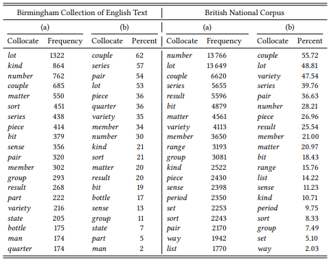
Renouf and Sinclair choose a different strategy: for each item, they calculate the percentage of all occurrences of that item within the collocational framework. The results are shown in the columns labeled (b) (for example, number occurrs in the BNC a total of 48 806 times, so the 13 799 times that it occurs in the pattern [a __ of ] account for 28.21 percent of its occurrences). As you can see, the order changes slightly, but the basic result appears to remain the same. Broadly speaking, the most strongly associated words in both corpora and by either measure tend to be related to quantities (e.g. lot, number,couple), part-whole relations (e.g. piece, member, group, part), or types (e.g. sort or variety). This kind of semantic coherence is presented by Renouf and Sinclair as evidence that collocational frameworks are relevant units of language.

Keeping this in mind, let us discuss the difference between frequency and percentages in some more detail. Note, first, that the reason the results do not change perceptibly is because Renouf and Sinclair do not determine the percentage of occurrences of words inside [a __ of ] for all words in the framework, but only for the twenty nouns that they have already identified as most frequent – the columns labeled (b) thus represent a ranking based on a mixed strategy of preselecting words by their raw frequency and then ranking them by their proportions inside and outside the framework.

If we were to omit the pre-selection stage and calculate the percentages for all words occurring in the framework – as we should, if these percentages are relevant – we would find 477 words in the BNC that occur exclusively in the framework, and thus all have an association strength of 100 percent – among them words that fit the proposed semantic preferences of the pattern, like barrelful, words that do not fit, like bomb-burst, hyserisation or Jesuitism, and many misspellings, like fct (for fact) and numbe and numbr (for number). The problem here is that percentages, like some other association measures, massively overestimate the importance of rare events. In order to increase the quality of the results, let us remove all words that occur five times or less in the BNC. The twenty words in Table 8.2 are then the words with the highest percentages of occurrence in the framework [a __ of ].

Table 8.2: The collocational framework [a __ of ] in the BNC by percentage of occurrences

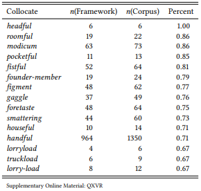
This list is obviously completely different from the one in Renouf & Sinclair (1991) or our replication. We would not want to call them typical for [a __ of ], in the sense that it is not very probable that we will encounter them in this collocational framework. However, note that they generally represent the same categories as the words in Table 8.1, namely ‘quantity’ and ‘part-whole’, indicating a relevant relation to the framework. This relation is, in fact, the counterpart to the one shown in Table 8.1: These are words for which the framework [a __ of ] is typical, in the sense that if we encounter these words, it is very probable that they will be accompanied by this collocational framework.

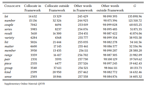
There are words that are typical for a particular framework, and there are frameworks that are typical for particular words; this difference in perspective may be of interest in particular research designs (cf. Stefanowitsch & Flach 2016 for further discussion). Generally, however, it is best to use an established association measure that will not overestimate rare events. Table 8.3 shows the fifteen most strongly associated words in the framework based on the G statistic.

Table 8.3: Top collocates of the collocational framework [a __ of ] (BNC)

This case study has introduced the notion of collocational frameworks as a simple way of studying the relationship between words and their grammatical context and the potential functional nature of this relationship. It is also meant as a reminder that different corpora and especially different measures of collocation strength will yield different results.

8.2.1.2 Case study: [there V_linksomething ADJ about NP]

As an example of a grammar pattern, consider [there V_link something ADJ about NP] (Hunston & Francis 2000: 105–106). As is typical of grammar patterns, this pattern constitutes a canonical unit of grammatical structure – unlike Renouf and Sinclair’s collocational frameworks.

Hunston and Francis mention this pattern only in passing, noting that it “has the function of evaluating the person or thing indicated in the noun group following about”. Their usual procedure (which they skip in this case) is to back up such observations concerning the meaning of grammar patterns by listing the most frequent items occurring in this pattern and showing that these form one or more semantic classes (similar to the procedure used by Renouf and Sinclair). In (1), I list all words occurring in the British National Corpus more than twice in the pattern under investigation, with their frequency in parentheses:

(1) odd (21), special (20), different (18), familiar (16), strange (13), sinister (8), disturbing (5), funny (5), wrong (5), absurd (4), appealing (4), attractive (4), fishy (4), paradoxical (4), sad (4), unusual (4), impressive (3), shocking (3), spooky (3), touching (3), unique (3), unsatisfactory (3)

The list clearly supports Hunston and Francis’s claim about the meaning of this grammar pattern – most of the adjectives are inherently evaluative. There are a few exceptions – different, special, unusual and unique do not have to be used evaluatively. If they occur in the pattern [there V_link something ADJ about NP], however, they are likely to be interpreted evaluatively.

As Hunston & Francis (2000: 105) point out: “Even when potentially neutral words such as nationality words, or words such as masculine and feminine, are used in this pattern, they take on an evaluative meaning”. This is, in fact, a crucial feature of grammar patterns, as it demonstrates that these patterns themselves are meaningful and are able to impart their meaning on words occurring in them. The following examples demonstrate this:

(2) a. There is something horribly cyclical about television advertising. (BNC CBC)

b. It is a big, square box, painted dirty white, and, although he is always knocking through, extending, repapering and spring-cleaning, there is something dead about the place. (BNC HR9)

c. At least it didn’t sound now quite like a typewriter, but there was something metallic about it. (BNC J54)

The adjective cyclical is neutral, but the adverb horribly shows that it is meant evaluatively in (2a); dead in its literal sense is purely descriptive, but when applied to things (like a house in 2b), it becomes an evaluation; finally, metallic is also neutral, but it is used to evaluate a sound negatively in (2c), as shown by the phrasing at least ... but.

Instead of listing frequencies, of course, we could calculate the association strength between the pattern [there V_link something ADJ about NP] and the adjectives occurring in it. I will discuss in more detail how this is done in the next subsection; for now, suffice it to say that it would give us the ranking in Table 8.4.

Table 8.4: Most strongly associated adjectives in the pattern [there V_link something ADJ about NP]

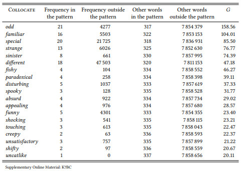
The ranking does not differ radically from the ranking by frequency in (2) above, but note that the descriptive adjectives special and different are moved down the list a few ranks and unique and unusual disappear from the top twenty, sharpening the semantic profile of the pattern.

This case study is meant to introduce the notion of grammar patterns and to show that these patterns often have a relatively stable meaning that can be uncovered by looking at the words that are frequent in (or strongly associated with) them. Like the preceding case study, it also introduced the idea that the relationship between words and units of grammatical structure can be investigated using the logic of association measures. The next sections look at this in more detail.

8.2.2 Collostructional analysis

Under the definition of corpus linguistics used throughout this book, there should be nothing surprising about the idea of investigating the relationship between words and units of grammatical structure based on association measures: a grammatical structure is just another condition under which we can observe the occurrence of lexical items. This is the basic idea of collostructional analysis, a methodological perspective first proposed in Stefanowitsch & Gries (2003), who refer to words that are associated with a particular construction a collexeme of that construction. Their perspective builds on ideas in collocation analysis, colligation analysis (cf. Section 8.2.4 below) and pattern grammar, but is more rigorously quantitative, and conceptually grounded in construction grammar. It has been applied in all areas of grammar, with a focus on argument structure (see Stefanowitsch & Gries (2009) and Stefanowitsch (2013) for overviews). Like collocation analysis, it is generally inductive, but it can also be used to test certain general hypotheses about the meaning of grammatical constructions.

8.2.2.1 Case study: The ditransitive

Stefanowitsch & Gries (2003) investigate, among other things, which verbs are strongly associated with the ditransitive construction (or ditransitive subcategorization, if you don’t like constructions). This is a very direct application of the basic research design for collocates introduced in the preceding chapter.

Their design is broadly deductive, as their hypothesis is that constructions have meaning and specifically, that the ditransitive has a ‘transfer’ meaning. The design has two nominal variables: ARGUMENT STRUCTURE (with the values DITRANSITIVE and OTHER) and VERB (with values corresponding to all verbs occurring in the construction). The prediction is that the most strongly associated verbs will be verbs of literal or metaphorical transfer. Table 8.5 gives the information needed to calculate the association strength for give (although the procedure should be familiar by now), and Table 8.6 shows the ten most strongly associated verbs.¹

Table 8.5: Give and the ditransitive (ICE-GB)

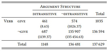
Table 8.6: The verbs in the ditransitive construction (ICE-GB, Stefanowitsch & Gries (2003: 229))

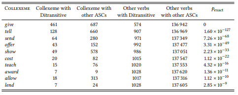
The hypothesis is corroborated: the top ten collexemes (and most of the other significant collexemes not shown here) refer to literal or metaphorical transfer.

However, note that on the basis of lists like that in Table 8.8 we cannot reject a null hypothesis along the lines of “There is no relationship between the ditransitive and the encoding of transfer events”, since we did not test this. All we can say is that we can reject null hypotheses stating that there is no relationship between the ditransitive and each individual verb on the list. In practice, this may amount to the same thing, but if we wanted to reject the more general null hypothesis, we would have to code all verbs in the corpus according to whether they are transfer verbs or not, and then show that transfer verbs are significantly more frequent in the ditransitive construction than in the corpus as a whole.

8.2.2.2 Case study: Ditransitive and prepositional dative

Collostructional analysis can also be applied in the direct comparison of two grammatical constructions (or other grammatical features), analogous to the differential collocate design discussed in Chapter 7. For example, Gries & Stefanowitsch (2004) compare verbs in the ditransitive and the so-called to-dative – both constructions express transfer meanings, but it has been claimed that the ditransitive encodes a spatially and temporally more direct transfer than the to-dative (Thompson & Koide 1987). If this is the case, it should be reflected in the verbs most strongly associated to one or the other construction in a direct comparison. Table 8.7 shows the data needed to determine for the verb give which of the two constructions it is more strongly attracted to.

Table 8.7: Give in the ditransitive and the prepositional dative (ICE-GB)

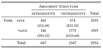
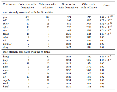
Give is significantly more frequent than expected in the ditransitive and less frequent than expected in the to-dative (p_exact = 1.8 × 10⁻¹²⁰). It is therefore said to be a significant distinctive collexeme of the ditransitive (again, I will use the term differential instead of distinctive in the following). Table 8.8 shows the top ten differential collexemes for each construction.

Generally speaking, the list for the ditransitive is very similar to the one we get if we calculate the simple collexemes of the construction; crucially, many of the differential collexemes of the to-dative highlight the spatial distance covered by the transfer, which is in line with what the hypothesis predicts.

8.2.2.3 Case study: Negative evidence

Recall from the introductory chapter that one of the arguments routinely made against corpus linguistics is that corpora do not contain negative evidence. Even corpus linguists occasionally agree with this claim. For example, McEnery & Wilson (2001: 11), in their otherwise excellent introduction to corpus-linguistic thinking, cite the sentence in (3):

(3) * He shines Tony books.

Table 8.8: Verbs in the ditransitive and the prepositional dative (ICE-GB, Gries & Stefanowitsch 2004: 106).

They point out that this sentence will not occur in any given finite corpus, but that this does not allow us to declare it ungrammatical, since it could simply be one of infinitely many sentences that “simply haven’t occurred yet”. They then offer the same solution Chomsky has repeatedly offered:

It is only by asking a native or expert speaker of a language for their opinion of the grammaticality of a sentence that we can hope to differentiate unseen but grammatical constructions from those which are simply grammatical but unseen (McEnery & Wilson 2001: 12).

However, as Stefanowitsch (2008; 2006b) points out, zero is just a number, no different in quality from 1, or 461 or any other frequency of occurrence. This means that any statistical test that can be applied to combinations of verbs and grammatical constructions (or any other elements of linguistic structure) that do occur together can also be applied to combinations that do not occur together. Table 8.9 shows this for the verb say and the ditransitive construction in the ICE-GB.

Table 8.9: The non-occurrence of say in the ditransitive (ICE-GB)

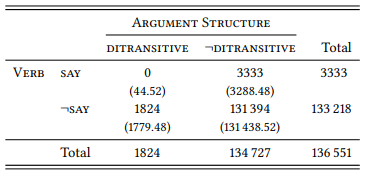
Fisher’s exact test shows that the observed frequency of zero differs significantly from that expected by chance (p = 4.3 × 10−165) (so does a χ² test: χ² = 46.25, df = 1, p < 0.001). In other words, it is very unlikely that sentences like Alex said Joe the answer “simply haven’t occurred yet” in the corpus. Instead, we can be fairly certain that say cannot be used with ditransitive complementation in English. Of course, the corpus data do not tell us why this is so, but neither would an acceptability judgment from a native speaker.

Table 8.10 shows the twenty verbs whose non-occurrence in the ditransitive is statistically most significant in the ICE-GB (see Stefanowitsch 2006b: 67). Since the frequency of co-occurrence is always zero and the frequency of other words in the construction is therefore constant, the order of association strength corresponds to the order of the corpus frequency of the words. The point of statistical testing in this case is to determine whether the absence of a particular word is significant or not.

Note that since zero is no different from any other frequency of occurrence, this procedure does not tell us anything about the difference between an intersection of variables that did not occur at all and an intersection that occurred with any other frequency less than the expected one. All the method tells us is whether an occurrence of zero is significantly less than expected.

Table 8.10: Non-occurring verbs in the ditransitive (ICE-GB)

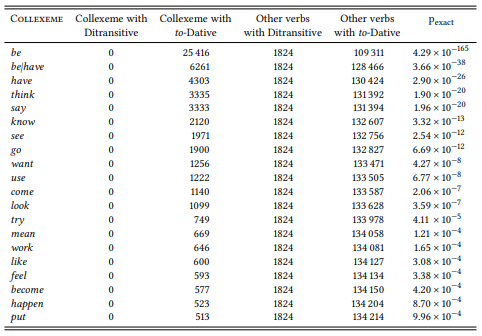
In other words, the method makes no distinction between zero occurrence and other less-frequent-than-expected occurrences. However, Stefanowitsch (2006b: 70f) argues that this is actually an advantage: if we were to treat an occurrence of zero as special opposed to, say, an occurrence of 1, then a single counterexample to an intersection of variables hypothesized to be impossible will appear to disprove our hypothesis. The knowledge that a particular intersection is significantly less frequent than expected, in contrast, remains relevant even when faced with apparent counterexamples. And, as anyone who has ever elicited acceptability judgments – from someone else or introspectively from themselves – knows, the same is true of such judgments: We may strongly feel that something is unacceptable even though we know of counterexamples (or can even think of such examples ourselves) that seem possible but highly unusual.

Of course, applying significance testing to zero occurrences of some intersection of variables is not always going to provide a significant result: if one (or both) of the values of the intersection are rare in general, an occurrence of zero may not be significantly less than expected. In this case, we still do not know whether the absence of the intersection is due to chance or to its impossibility – but with such rare combinations, acceptability judgments are also going to be variable.

8.2.3 Words and their grammatical properties

Studies that take a collocational perspective on associations between words and grammatical structure tend to start from one or more grammatical structures and inductively identify the words associated with these structures. Moving away from this perspective, we find research designs that begin to resemble more closely the kind illustrated in Chapters 5 and 6, but that nevertheless include lexical items as one of their variables. These designs will typically start from a word (or a small set of words) and identify associated grammatical (structural and semantic) properties. This is of interest for many reasons, for example in the context of how much idiosyncrasy there is in the grammatical behavior of lexical items in general (for example, what are the grammatical differences between near synonyms), or how much of a particular grammatical alternation is lexically determined.

8.2.3.1 Case study: Complementation of begin and start

There are a number of verbs in English that display variation with respect to their complementation patterns, and the factors influencing this variation have provided (and continue to provide) an interesting area of research for corpus linguists. In an early example of such a study, Schmid (1996) investigates the near-synonyms begin and start, both of which can occur with to-clauses or ing-clauses, as shown in (4a–d):

(4) a. It rained almost every day, and she began to feel imprisoned. (BNC A7H)

b. [T]here was a slightly strained period when he first began working with the group... (BNC AT1)

c. The baby wakened and started to cry. (BNC CB5)

d. Then an acquaintance started talking to me and diverted my attention. (BNC ABS)

Schmid’s study is deductive. He starts by deriving from the literature two hypotheses concerning the choice between the verbs begin and start on the one hand and to- and the ing-complements on the other: First, that begin signals gradual onsets and start signals sudden ones, and second, that ing-clauses are typical of dynamic situations while to-clauses are typical of stative situations.

His focus is on the second hypothesis, which he tests on the LOB corpus by, first, identifying all occurrences of both verbs with both complementation patterns and, second, categorizing them according to whether the verb in the complement clause refers to an activity, a process or a state. The study involves three nominal variables: MATRIX VERB (with the values BEGIN and START), Complementation (with the values ING-clause and TO-clause) and AKTIONSART (with the values ACTIVITY, PROCESS and STATE). Thus, we are dealing with a multivariate design. The prediction with respect to the complementation pattern is clear – to-complements should be associated with activities and ing-complements with states, with processes falling somewhere in between. There is no immediate prediction with respect to the choice of verb, but Schmid points out that activities are more likely to have a sudden onset, while states and processes are more likely to have a gradual onset, thus the former might be expected to prefer start and the latter begin.

Schmid does not provide an annotation scheme for the categories activity, process and state, discussing these crucial constructs in just one short paragraph:

Essentially, the three possible types of events that must be considered in the context of a beginning are activities, processes and states. Thus, the speaker may want to describe the beginning of a human activity like eating, working or singing; the beginning of a process which is not directly caused by a human being like raining, improving, ripening; or the beginning of a state. Since we seem to show little interest in the beginning of concrete, visible states (cf. e.g. ^?The lamp began to stand on the table.) the notion of state is in the present context largely confined to bodily, intellectual and emotive states of human beings. Examples of such “private states” (Quirk et al. 1985: 202f) are being ill, understanding, loving.

Quirk et al. (1985: 202–203) mention four types of “private states”: intellectual states, like know, believe, realize; states of emotion or attitude, like intend, want, pity; states of perception, like see, smell, taste; and states of bodily sensation, like hurt, itch, feel cold. Based on this and Schmid’s comments, we might come up with the following rough annotation scheme which thereby becomes our operationalization for AKTIONSART:

(5) A simple annotation scheme for AKTIONSART

a. ACTIVITY: any externally perceivable event under the control of an animate agent.

b. PROCESS: any externally perceivable event not under the control of an animate agent, including events involving involuntary animate themes (like cry, menstruate, shiver) and events not involving animate entities.

c. STATE: any externally not perceivable event involving human cognition, as well as unchanging situations not involving animate entities.

Schmid also does not state how he deals with passive sentences like those in (6a, b):

(6) a. [T]he need for correct and definite leadership began to be urgently felt... (LOB G03)

b. Presumably, domestic ritual objects began to be made at much the same time. (LOB J65)

These could be annotated with reference to the grammatical subject; in this case they would always be processes, as passive subjects are never voluntary agents of the event described. Alternatively, they could be annotated with reference to the logical subject, in which case (6a) would be a state (‘someone feels something’) and (6b) would be an activity (‘someone makes domestic ritual objects’). Let us choose the second option here.

Querying (7a, b) yields 348 hits (Schmid reports 372, which corresponds to the total number of hits for these verbs in the corpus, including those with other kinds of complementation):

(7) a. [lemma="(begin|start)"] [pos="verb_pres.part."]

b. [lemma="(begin|start)"] [word="to"%c] [pos="verb_infinitive"]

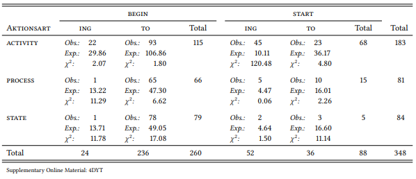
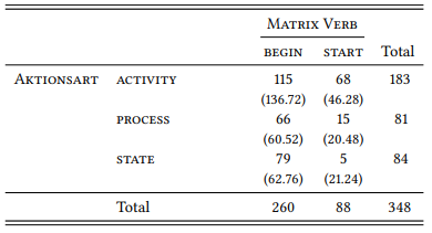
Annotating all 348 hits according to the annotation scheme sketched out above yields the data in Table 8.11 (the complete annotated concordance is part of the Supplementary Online Material). The total frequencies as well as the proportions among the categories differ slightly from the data Schmid reports, but the results are overall very similar.

As always in a configural frequency analysis, we have to correct for multiple testing: there are twelve cells in our table, so our probability of error must be lower than ^0.05/₁₂ = 0.0042. The individual cells (i.e., intersections of variables) have one degree of freedom, which means that our critical χ² value is 8.20. This means that there are two types and three antitypes that reach significance: as predicted, activity verbs are positively associated with the verb start in combination with ing-clauses and state verbs are positively associated with the verb begin in combination with to-clauses. Process verbs are also associated with begin with to-clauses, but only marginally significantly so. As for the antitypes, all three verb classes are negatively associated (i.e., less frequent than expected) with the verb begin with ing-clauses, which suggests that this complementation pattern is generally avoided with the verb begin, but this avoidance is particularly pronounced with state and process verbs, where it is statistically significant: the verb begin and state/process verbs both avoid ing-complementation, and this avoidance seems to add up when they are combined.

Table 8.11: Aktionsart, matrix verb and complementation type (LOB)

Faced with these results, we might ask, first, how they relate to two simpler tests of Schmid’s hypothesis – namely two bivariate designs separately testing (a) the relationship between AKTIONSART and COMPLEMENTATION, (b) the relationship between AKTIONSART and MATRIX VERB and (c) the relationship between MATRIX VERB and COMPLEMENTATION TYPE. We have all the data we need to test this in Table 8.11, we just have to sum up appropriately. Table 8.12 shows that AKTIONSART and COMPLEMENTATION TYPE are related: ACTIVITY VERBS prefer ING, the other two verb types prefer to (χ² = 49.702, df = 2, p < 0.001 )

Table 8.12: Aktionsart and complementation type (LOB)

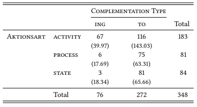
Table 8.13 shows that AKTIONSART and MATRIX VERB are also related: ACTIVITY verbs prefer TO and STATE verbs prefer ing (χ² = 32.236, df = 2, p < 0.001).

Table 8.13: Aktionsart and matrix verb (LOB)

Finally, Table 8.14 shows that MATRIX VERB and COMPLEMENTATION TYPE are also related: BEGIN prefers TO and START prefers ing (χ² = 95.755, df = 1, p < 0.001).

Table 8.14: Matrix verb and complementation type

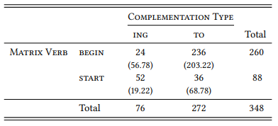
In other words, every variable in the design is related to every other variable and the multivariate analysis in Table 8.11 shows that the effects observed in the individual bivariate designs simply add up when all three variables are investigated together. Thus, we cannot tell whether any of the three relations between the variables is independent of the other two. In order to determine this, we would have to keep each of the variables constant in turn to see whether the other two still interact in the predicted way (for example, whether begin prefers to-clauses and start prefers ing-clauses even if we restrict the analysis to activity verbs, etc.

The second question we could ask faced with Schmid’s results is to what extent his second hypothesis – that begin is used with gradual beginnings and start with sudden ones – is relevant for the results. As mentioned above, it is not tested directly, so how could we remedy this? One possibility is to look at each of the 348 cases in the sample and try to determine the gradualness or suddenness of the beginning they denote. This is sometimes possible, as in (4a) above, where the context suggests that the referent of the subject began to feel imprisoned gradually the longer the rain went on, or in (4c), which suggests that the crying began suddenly as soon as the baby woke up. But in many other cases, it is very difficult to judge, whether a beginning is sudden or gradual – as in (4b, c). To come up with a reliable annotation scheme for this categorization task would be quite a feat.

There is an alternative, however: speakers sometimes use adverbs that explicitly refer to the type of beginning. A query of the BNC for〈 [word=".*ly"%c] [hw="(begin|start)"] 〉yields three relatively frequent adverbs (occurring more than 10 times) indicating suddenness (immediately, suddenly and quickly), and three indicating gradualness (slowly, gradually and eventually). There are more, like promptly, instantly, rapidly. leisurely, reluctantly, etc., which are much less frequent.

By extracting just these cases, we can directly test the hypothesis that begin signals gradual and start sudden onsets. The BNC contains 307 cases of [begin/ start to V_inf] and [begin/start Ving] directly preceded by one of the six adverbs mentioned above. Table 8.15 shows the result of a configural frequency analysis of the variables ONSET (SUDDEN vs. GRADUAL, MATRIX VERB (BEGIN vs. START and COMPLEMENTATION TYPE (ING vs. TO).

Table 8.15: Adverbs of suddenness and gradualness, matrix verb and complementation type

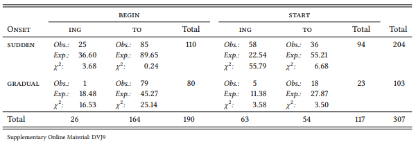
Since there are eight cells in the table, the corrected p -value is ^0.05/₈ = 0.00625; the individual cells have one degree of freedom, so the critical χ² value is 7.48. There are two significant types: sudden ∩ start ∩ ing and gradual ∩ begin ∩ to. There is one significant and one marginally significant antitype: sudden ∩ start ∩ to and gradual ∩ begin ∩ ing, respectively. This corroborates the hypothesis that begin signals gradual onsets and start signals sudden ones, at least when the matrix verbs occur with their preferred complementation pattern.

Summing up the results of both studies, we could posit two “prototype” patterns (in the sense of cognitive linguistics): [begin_gradual V ^stative _ing] and [startsudden to V ^activity _inf], and we could hypothesize that speakers will choose the pattern that matches most closely the situation they are describing (something that could then be tested, for example, in a controlled production experiment).

This case study demonstrated a complex design involving grammar, lexis and semantic categories. It also demonstrated that semantic categories can be included in a corpus linguistic design in the form of categorization decisions on the basis of an annotation scheme (in which case, of course, the annotation scheme must be documented in sufficient detail for the study to be replicable), or in the form of lexical items signaling a particular meaning explicitly, such as adverbs of gradualness (in which case we need a corpus large enough to contain a sufficient number of hits including these items). It also demonstrated that such corpus-based studies may result in very specific hypotheses about the function of lexicogrammatical structures that may become the basis for claims about mental representation.

8.2.4 Grammar and context

There is a wide range of contextual factors that are hypothesized or known to influence grammatical variation. These include information status, animacy and length, which we already discussed in the case studies of the possessive constructions in Chapters 5 and 6. Since we have dealt with them in some detail, they will not be discussed further here, but they have been extensively studied for a range of phenomena (e.g. Thompson & Koide 1987 for the dative alternation; Chen 1986 and Gries 2003b for particle placement; Rosenbach 2002 and Stefanowitsch 2003 for the possessives). Instead, we will discuss some less frequently investigated contextual factors here, namely word frequency, phonology, the “horror aequi” and priming.

8.2.4.1 Case study: Adjective order and frequency

In a comprehensive study on adjective order already mentioned in Chapter 4, Wulff (2003) studies (among other things) the hypothesis that in noun phrases with two adjectives, more frequent adjectives precede less frequent ones. There are two straightforward ways of testing this hypothesis. First (as Wulff does), based on mean frequencies: if we assume that the hypothesis is correct, then the mean frequency of the first adjective of two-adjective pairs should be higher than that of the second. Second, based on the number of cases in which the first and second adjective, respectively, are more frequent: if we assume that the hypothesis is correct, there should be more cases where the first adjective is the more frequent one than cases where the second adjective is the more frequent one. Obviously, the two ways of investigating the hypothesis could give us different results.

Let us replicate part of Wulff’s study using the spoken part of the BNC (Wulff uses the entire BNC). If we extract all sequences of exactly two adjectives occurring before a noun (excluding comparatives and superlatives), and include only those adjective pairs that (a) occur at least five times, and (b) do not occur more than once in the opposite order, we get the sample in Table 8.16 (the adjective pairs are listed in decreasing order of their frequency of occurrence). The table also lists the frequency of each adjective in the spoken part of the BNC (case insensitive), and, in the final column, states whether the first or the second adjective is more frequent.

Let us first look at just the ten most frequent adjective pairs (Ranks 1–10). The mean frequency of the first adjective is 5493.2, that of the second adjective is 4042.7. Pending significance testing, this would corroborate Wulff’s hypothesis. However, in six of these ten cases the second adjective is actually more frequent than the first, which would contradict Wulff’s hypothesis. The problem here is that some of the adjectives in first position, like good and right, are very frequent while some adjectives in second position, like honorable and northern are very infrequent – this influences the mean frequencies substantially. However, when comparing the frequency of the first and second adjective, we are making a binary choice concerning which of the adjectives is more frequent – we ignore the size of the difference.

If we look at the ten next most frequent adjectives, we find the situation reversed – the mean frequency is 3672.3 for the first adjective and 4072 for the second adjective, contradicting Wulff’s hypothesis, but in seven of the ten cases, the first adjective is more frequent, corroborating Wulff’s hypothesis.

Table 8.16: Sample of [ADJ₁ ADJ₂ ] sequences (BNC Spoken)

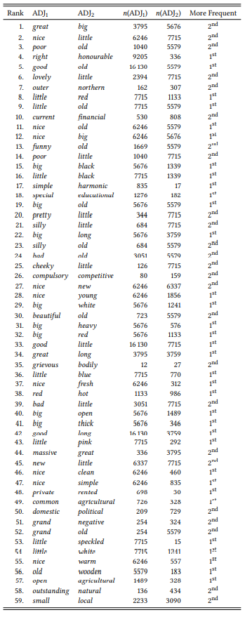
Both ways of looking at the issue have disadvantages. If we go by mean frequency, then individual cases might inflate the mean of either of the two adjectives. In contrast, if we go by number of cases, then cases with very little difference in frequency count just as much as cases with a vast difference in frequency. In cases like this, it may be advantageous to apply both methods and reject the null hypothesis only if both of them give the same result (and of course, our sample should be larger than ten cases).

Let us now apply both perspectives to the entire sample in Table 8.16, beginning with mean frequency. The mean frequency of the first adjective is 4371.14 with a standard deviation of 3954.22, the mean frequency of the second adjective is 3070.98 with a standard deviation of 2882.04. Using the formulas given in Chapter 6, this gives us a t -value of 2.04 at 106.06 degrees of freedom, which means that the difference is significant (p < 0.05). This would allow us to reject the null hypothesis and thus corroborates Wulff’s hypothesis.

Next, let us look at the number of cases that match the prediction. There are 34 cases where the first adjective is more frequent, and 25 cases where the second adjective is more frequent, which seems to corroborate Wulff’s hypothesis, but as Table 8.17 shows, the difference is not statistically significant.

Table 8.17: Adjective order and frequency (cf. Table 8.16)

Thus, we should be careful to conclude, based on our sample, that there is an influence of word frequency on adjective order. Although the results are encouraging, we would have to study a larger sample (Wulff (2003) does so and shows that, indeed, there is an influence of frequency on order).

This case study was meant to demonstrate that sometimes we can derive different kinds of quantitative predictions from a hypothesis which may give us different results; in such cases, it is a good idea to test all predictions. The case study also shows that word frequency may have effects on grammatical variation, which is interesting from a methodological perspective because not only is corpus linguistics the only way to test for such effects, but corpora are also the only source from which the relevant values for the independent variable can be extracted.

8.2.4.2 Case study: Binomials and sonority

Frozen binomials (i.e. phrases of the type flesh and blood, day and night, size and shape) have inspired a substantial body of research attempting to uncover principles determining the order of the constituents. A number of semantic, syntactic and phonological factors have been proposed and investigated using psycholinguistic and corpus-based methods (see Lohmann (2013) for an overview and a comprehensive empirical study). A phonological factor that we will focus on here concerns the sonority of the final consonants of the two constituents: it has been proposed that words with less sonorant final consonants occur before words with more sonorant ones (e.g. Cooper & Ross 1975).

In order to test this hypothesis, we need a sample of binomials. In the literature, such samples are typically taken from dictionaries or similar lists assembled for other purposes, but there are two problems with this procedure. First, these lists contain no information about the frequency (and thus, importance) of the individual examples. Second, these lists do not tell us exactly how “frozen” the phrases are; while there are cases that seem truly non-reversible (like flesh and blood), others simply have a strong preference (day and night is three times as frequent as night and day in the BNC) or even a relatively weak one (size and shape is only one-and-a-half times as frequent as shape and size). It is possible that the degree of frozenness plays a role – for example, it would be expected that binomials that never (or almost never) occur in the opposite order would display the influence of any factor determining order more strongly than those where the two possible orders are more equally distributed.

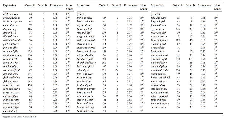
We can avoid these problems by drawing our sample from the corpus itself. For this case study, let us select all instances of [NOUN and NOUN] that occur at least 30 times in the BNC. Let us further limit our sample to cases where both nouns are monosyllabic, as it is known from the existing research literature that length and stress patterns have a strong influence on the order of binomials. Let us also exclude cases where one or both nouns are in the plural, as we are interested in the influence of the final consonant, and it is unclear whether this refers to the final consonant of the stem or of the word form.

This will give us the 78 expressions in Table 8.18. Next, let us calculate the degree of frozenness by checking for each binomial how often the two nouns occur in the opposite order. The proportion of the more frequent order can then be taken as representing the frozenness of the binomial – it will be 1 for cases where the order never varies and 0.5 for cases where the two orders are equally frequent, with most cases falling somewhere in between.

Table 8.18: Sample of monosyllabic binomials and their sonority

Finally, we need to code the final consonants of all nouns for sonority and determine which of the two final consonants is more sonorant – that of the first noun, or that of the second. For this, let us use the following (hopefully uncontroversial) sonority hierarchy:

(8) [vowels] > [semivowels] > [liquids] > [h] > [nasals] > [voiced fricatives] > [voiceless fricatives] > [voiced affricates] > [voiceless affricates] > [voiced stops] > [voiceless stops]

The result of all these steps is shown in Table 8.18. The first column shows the binomial in its most frequent order, the second column gives the frequency of the phrase in this order, the third column gives the frequency of the less frequent order (the reversal of the one shown), the fourth column gives the degree of frozenness (i.e., the percentage of the more frequent order), and the fifth column records whether the final consonant of the first or of the second noun is less sonorant.

Let us first simply look at the number of cases for which the claim is true or false. There are 42 cases where the second word’s final consonant is more sonorant than that of the second word (as predicted), and 36 cases where the second word’s final consonant is less sonorant than that of the first (counter to the prediction). As Table 8.19 shows, this difference is nowhere near significant.

Table 8.19: Sonority of the final consonant and word order in binomials (counts)

However, note that we are including both cases with a very high degree of frozenness (like beck and call, flesh and blood, or lock and key) and cases with a relatively low degree of frozenness (like nose and mouth, day and night, or snow and ice: this will dilute our results, as the cases with low frozenness are not predicted to adhere very strongly to the less-before-more-sonorant principle.

We could, of course, limit our analysis to cases with a high degree of frozenness, say, above 90 percent (the data is available, so you might want to try). However, it would be even better to keep all our data and make use of the rank order that the frozenness measure provides: the prediction is that cases with a high frozenness rank will adhere to the sonority constraint with a higher probability than those with a low frozenness rank. Table 8.18 contains all the data we need to determine the median of words adhering or not adhering to the constraint, as well as the rank sums and number of cases, which we need to calculate a U -test. We will not go through the test step by step (but you can try for yourself if you want to). Table 8.20 provides the necessary values derived from Table 8.18.

Table 8.20: Sonority of the final consonant and word order in binomials (ranks)

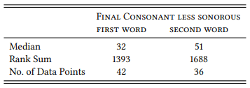
The binomials adhering to the less-before-more-sonorant principle have a much higher median frozenness rank than those not adhering to the constraint – in other words, binomials with a high degree of frozenness tend to adhere to the constraint, binomials with a low degree of frozenness do not. The U -test shows that the difference is highly significant (U = 490, N₁ = 36, N₂ = 42, p < 0.001).

Like the case study in Section 8.2.4.1, this case study was intended to show that sometimes we can derive different kinds of quantitative predictions from a hypothesis; however, in this case one of the possibilities more accurately reflects the hypothesis and is thus the one we should base our conclusions on. The case study was also meant to provide an example of a corpus-based design where it is more useful to operationalize one of the constructs (Frozenness) as an ordinal, rather than a nominal variable. In terms of content, it was meant to demonstrate how phonology can interact with grammatical variation (or, in this case, the absence of variation) and how this can be studied on the basis of corpus data; cf. Schlüter (2003) for another example of phonology interacting with grammar, and cf. Lohmann (2013) for a comprehensive study of binomials.

8.2.4.3 Case study: Horror aequi

In a number of studies, Günter Rohdenburg and colleagues have studied the influence of contextual (and, consequently, conceptual) complexity on grammatical variation (e.g. Rohdenburg 1995; 2003). The general idea is that in contexts that are already complex, speakers will try to choose a variant that reduces (or at least does not contribute further to) this complexity. A particularly striking example of this is what Rohdenburg (adapting a term from Karl Brugmann) calls the horror aequi principle: “the widespread (and presumably universal) tendency to avoid the repetition of identical and adjacent grammatical elements or structures” (Rohdenburg 2003: 206).

Take the example of matrix verbs that normally occur alternatively with a to-clause or an ing-clause (like begin and start in Case Study 8.2.3.1 above). Rohdenburg (1995: 380) shows, on the basis of the text of an 18th century novel, that where such matrix verbs occur as to-infinitives, they display a strong preference for ing-complements. For example, in the past tense, start freely occurs either with a to-complement, as in (9a) or with an ing-complement, as in (9b). However, as a to-infinitive it would avoid the to-complement, although not completely, as (9c) shows, and strongly prefer the ing-form, as in (9d):

(9) a. I started to think about my childhood again... (BNC A0F)

b. So I started thinking about alternative ways to earn a living... (BNC C9H)

c. ... in the future they will actually have to start to think about a fairer electoral system... (BNC JSG)

d. He will also have to start thinking about a partnership with Skoda before (BNC A6W)

Impressionistically, this seems to be true: in the BNC there are 11 cases of started to think about, 18 of started thinking about, only one of to start to think about but 35 of to start thinking about.

Let us attempt a more comprehensive analysis and look at all cases of the verb start with a clausal complement in the BNC. Since we are interested in the influence of the tense/aspect form of the verb start on complementation choice, let us distinguish the inflectional forms start (base form), starts (3rd person), started (past tense/past participle) and starting (present participle); let us further distinguish cases of the base form start with and without the infinitive marker to (we can derive the last two figures by first searching for (10a) and (10b) and then for (10c) and (10d), and then subtracting the frequencies of the latter two from those of the former two, respectively:

(10) a. [word="start"%c] [word="to"%c]

b. [word="start"%c] [word=".*ing"%c]

c. [word="to"%c] [word="start"%c] [word="to"%c]

d. [word="to"%c] [word="start"%c] [word=".*ing"%c]

Table 8.21 shows the observed and expected frequencies of to- and ing-complements for each of these forms, together with the expected frequencies and the χ² components

Table 8.21: Complementation of start and the horror aequi principle

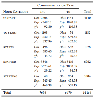
e most obvious and, in terms of their χ² components, most significant deviations from the expected frequencies are indeed those cases where the matrix verb start has the same form as the complement clause: there are far fewer cases of [to start to V_inf] and [starting V_pres.part.] and, conversely, far more cases of [to start V_pres.part.] and [starting to V_inf] than expected. Interestingly, if the base form of start does not occur with an infinitive particle, the to-complement is still strongly avoided in favor of the ing-complement, though not as strongly as in the case of the base form with the infinitive particle. It may be that horror aequi is a graded principle – the stronger the similarity, the stronger the avoidance.

This case study is intended to introduce the notion of horror aequi, which has been shown to influence a number of grammatical and morphological variation phenomena (cf. e.g. Rohdenburg 2003, Vosberg 2003, Rudanko 2003, Gries & Hilpert 2010). Methodologically, it is a straightforward application of the χ² test, but one where the individual cells of the contingency table and their χ² values are more interesting than the question whether the observed distribution as a whole differs significantly from the expected one.

8.2.4.4 Case study: Synthetic and analytic comparatives and persistence

The horror aequi principle has been shown to have an effect on certain kinds of variation and it can plausibly be explained as a way of reducing complexity (if the same structure occurs twice in a row, this might cause problems for language processing). However, there is another well-known principle that is, in a way, the opposite of horror aequi: structural priming. The idea of priming comes from psychology, where it refers to the fact that the response to a particular stimulus (the target) can be influenced by a preceding stimulus (the prime). For example, if subjects are exposed to a sequence of two pictures, they will identify an object on the second picture (say, a loaf of bread) faster and more accurately if it is related to the the scene in the first picture (say, a kitchen counter) (cf. Palmer 1975). Likewise, they will be faster to recognize a string of letters (say, BUTTER) as a word if it is preceded by a related word (say, BREAD) (cf. Meyer & Schvaneveldt 1971).

Bock (1986)shows that priming can also be observed in the production of grammatical structures. For example, if people read a sentence in the passive and are then asked to describe a picture showing an unrelated scene, they will use passives in their description more frequently than expected. She calls this structural priming. Interestingly, such priming effects can also be observed in naturally occurring language, i.e. in corpora (see Gries 2005 and Szmrecsanyi 2005; 2006) – if speakers use a particular syntactic structure, this increases the probability that they will use it again within a relatively short span.

For example, Szmrecsanyi (2005) argues that persistence is one of the factors influencing the choice of adjectival comparison. While most adjectives require either synthetic comparison (further, but not *more far) or analytic comparison (more distant, but not *distanter), some vary quite freely between the two (friendlier/more friendly). Szmrecsanyi hypothesizes that one of many factors influencing the choice is the presence of an analytic comparative in the directly preceding context: if speakers have used an analytic comparative (for example, with an adjective that does not allow anything else), this increases the probability that they will use it within a certain span with an adjective that would theoretically also allow a synthetic comparison. Szmrecsanyi shows that this is the case, but that it depends crucially on the distance between the two instances of comparison: the persistence is rather short-lived.

Let us attempt to replicate his findings in a small analysis focusing only on persistence and disregarding other factors. Studies of structural priming have two nominal variables: the PRIME, a particular grammatical structure occurring in a discourse, and the TARGET, the same (or a similar) grammatical structure occurring in the subsequent discourse. In our case, the grammatical structure is COMPARATIVE with the two values ANALYTIC and SYNTHETIC. In order to determine whether priming occurs and under what conditions, we have to extract a set of potential targets and the directly preceding discourse from a corpus. The hypothesis is always that the value of the prime will correlate with the value of the target – in our case, that analytic comparatives have a higher probability of occurrence after analytic comparatives and synthetic comparatives have a higher probability of occurrence after synthetic comparatives.

For our purposes, let us include only adjectives with exactly two syllables, as length and stress pattern are known to have an influence on the choice between the two strategies and must be held constant in our design. Let us further focus on adjectives with a relatively even distribution of the two strategies and include only cases where the less frequent comparative form accounts for at least forty percent of all comparative forms. Finally, let us discard all adjectives that occur as comparatives less than 20 times in the BNC. This will leave just six adjectives: angry, empty, friendly, lively, risky and sorry.

Let us extract all synthetic and analytic forms of these adjectives from the BNC. This will yield 452 hits, of which two are double comparatives (more livelier), which are irrelevant to our design and must be discarded. This leaves 450 potential targets – 241 analytic and 209 synthetic. Of these, 381 do not have an additional comparative form in a span of 20 tokens preceding the comparative – whatever determined the choice between analytic and synthetic comparatives in these cases, it is not priming. These non-primed comparatives are fairly evenly distributed – 194 are analytic comparatives and 187 are synthetic, which is not significantly different from a chance distribution (χ² = 0.13, df = 1, p = 0.7199), suggesting that our sample of adjectives does indeed consist of cases that are fairly evenly distributed across the two comparative strategies (see Supplementary Online Material for the complete annotated concordance).

Let us extract all synthetic and analytic forms of these adjectives from the BNC. This will yield 452 hits, of which two are double comparatives (more livelier), which are irrelevant to our design and must be discarded. This leaves 450 potential targets – 241 analytic and 209 synthetic. Of these, 381 do not have an additional comparative form in a span of 20 tokens preceding the comparative – whatever determined the choice between analytic and synthetic comparatives in these cases, it is not priming. These non-primed comparatives are fairly evenly distributed – 194 are analytic comparatives and 187 are synthetic, which is not significantly different from a chance distribution (χ² = 0.13, df = 1, p = 0.7199), suggesting that our sample of adjectives does indeed consist of cases that are fairly evenly distributed across the two comparative strategies (see Supplementary Online Material for the complete annotated concordance).

This leaves 69 targets that are preceded by a comparative prime in the preceding span of 20 tokens. Table 8.22 shows the distribution of analytic and synthetic primes and targets (if there was more than one comparative in the preceding context, only the one closer to the comparative in question was counted).

Table 8.22: Comparatives preceding comparatives in a context of 20 tokens (BNC)

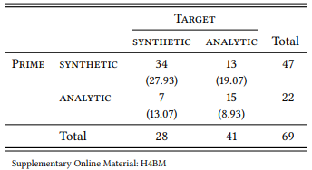
There is a significant influence of PRIME on TARGET: synthetic comparatives are more frequent than expected following synthetic comparatives, and analytic comparatives are more frequent than expected following analytic comparatives (χ² = 10.205, df = 1, p < 0.01). The effect is only moderate (�� = 0.3846), but note that the context within which we looked for potential primes is quite large – in some cases, the prime will be quite far away from the target, as in (11a), in other cases it is very close, as in (11b):

(11)     a. But the statistics for the second quarter, announced just before the October Conference of the Conservative Party, were even more damaging to the                    Government showing a rise of 17 percent on 1989. Indeed these figures made even sorrier reading for the Conservatives when one realized... (BNC G1J)

   b. Over the next ten years, China will become economically more liberal, internationally more friendly... (BNC ABD)

Obviously, we would expect a much stronger priming effect in a situation like that in (11b), where one word intervenes between the two comparatives, than in a situation like (11a), where 17 words (and a sentence boundary) intervene. Let us therefore restrict the context in which we count analytic comparatives to a size more likely to lead to a priming effect – say, seven words (based on the factoid that short term memory can hold up to seven units). Table 8.23 shows the distribution of primes and targets in this smaller window.

Table 8.23: Comparatives preceding comparatives in a context of 7 tokens (BNC)

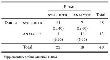
Again, the effect is significant (χ² = 15.08, df = 1, p < 0.001), but crucially, the effect size has increased noticeably to ϕ = 0.6141. This suggests that the structural priming effect depends quite strongly on the distance between prime and target.

This case study demonstrates structural priming (cf. Szmrecsanyi (2005) for additional examples) and shows how it can be studied on the basis of corpora. It also demonstrates that slight adjustments in the research design can have quite substantial effects on the results.

8.2.5 Variation and change

8.2.5.1 Case study: Sex differences in the use of tag questions

Grammatical differences may also exist between varieties spoken by subgroups of speakers defined by demographic variables, for example, when the speech of younger speakers reflects recent changes in the language, or when speakers from different educational or economic backgrounds speak different established sociolects. Even more likely are differences in usage preference. For example, Lakoff (1973) claims that women make more intensive use of tag questions than men. Mondorf (2004b) investigates this claim in detail on the basis of the London-Lund Corpus, which is annotated for intonation among other things. Mondorf’s analysis not only corroborates the claim that women use tag questions more frequently than men, but also shows qualitative differences in terms of their form and function.

This kind of analysis requires very careful, largely manual data extraction and annotation so it is limited to relatively small corpora, but let us see what we can do in terms of a larger-scale analysis. Let us focus on tag questions with negative polarity containing the auxiliary be (e.g. isn’t it, wasn’t she, am I not, was it not). These can be extracted relatively straightforwardly even from an untagged corpus using the following queries:

(12)     a. [word="(am|are|is|was|were)"%c] [word="n't"%c] [word="(I| you|he|she|it|we|they)"%c] [word="[.,!?]"]

   b. [word="(am|are|is|was|were)"%c] [word="(I|you|he|she|it| we|they)"%c] [word="not"%c] [word="[.,!?]"]

The query in (12a) will find all finite forms of the verb be (as non-finite forms cannot occur in tag questions), followed by the negative clitic n’t, followed by a pronoun; the query in (12b) will do the same thing for the full form of the particle not, which then follows rather than precedes the pronoun. Both queries will only find those cases that occur before a punctuation mark signaling a clause boundary (what to include here will depend on the transcription conventions of the corpus, if it is a spoken one).

The queries are meant to work for the spoken portion of the BNC, which uses the comma for all kinds of things, including hesitation or incomplete phrases, so we have to make a choice whether to exclude it and increase the precision or to include it and increase the recall (I will choose the latter option). The queries are not perfect yet: British English also has the form ain’t it, so we might want to include the query in (13a). However, ain’t can stand for be or for have, which lowers the precision somewhat. Finally, there is also the form innit in (some varieties of) British English, so we might want to include the query in (13b). However, this is an invariant form that can occur with any verb or auxiliary in the main clause, so it will decrease the precision even further. We will ignore ain’t and innit here (they are not particularly frequent and hardly change the results reported below):

(13)     a. [word="ai"%c] [word="n't"%c]

       [word="(I|you|he|she|it|we|they)"%c] [word="[.,!?]"]

   b. [word="in"%c] [word="n"%c] [word="it"%c] [word="[.,!?]"]

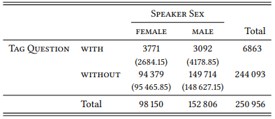
In the part of the spoken BNC annotated for speaker sex, there are 3751 hits for the patterns in (12a,b) for female speakers (only 20 of which are for 12b), and 3050 hits for male speakers (only 42 of which are for 12b). Of course, we cannot assume that there is an equal amount of male and female speech in the corpus, so the question is what to compare these frequencies against. Obviously, such tag questions will normally occur in declarative sentences with positive polarity containing a finite form of be. Such sentences cannot be retrieved easily, so it is difficult to determine their precise frequency, but we can estimate it. Let us search for finite forms of be that are not followed by a negative clitic (isn’t) or particle (is not) within the next three tokens (to exclude cases where the particle is preceded by an adverb, as in is just/obviously/... not). There are 146 493 such occurrences for female speakers and 215 219 for male speakers. The query will capture interrogatives, imperatives, subordinate clauses and other contexts that cannot contain tag questions, so let us draw a sample of 100 hits from both samples and determine how many of the hits are in fact declarative sentences with positive polarity that could (or do) contain a tag question. Let us assume that we find 67 hits in the female-speaker sample and 71 hits in the male-speaker sample to be such sentences. We can now adjust the total results of our queries by multiplying them with 0.67 and 0.71 respectively, giving us 98 150 sentences for female and 152 806 sentences for male speakers. In other words, male speakers produce 60.89 percent of the contexts in which a negative polarity tag question with be could occur. We can cross-check this by counting the total number of words uttered by male and female speakers in the spoken part of the BNC: there are 5 654 348 words produced by men and 3 825 804 words produced by women, which means that men produce 59.64 percent of the words, which fits our estimate very well.

These numbers can now be used to compare the number of tag questions against, as shown in Table 8.24. Since the tag questions that we found using our queries have negative polarity, they are not included in the sample, but must occur as tags to a subset of the sentences. This means that by subtracting the number of tag questions from the total for each group of speakers, we get the number of sentences without tag questions.

The difference between male and female speakers is highly significant, with female speakers using substantially more tag questions than expected, and male speakers using substantially fewer (χ² = 743.07, df = 1, p < 0.001).

This case study was intended to introduce the study of sex-related differences in grammar (or grammatical usage); cf. Mondorf (2004a) for additional studies and an overview of the literature. It was also intended to demonstrate the kinds of steps necessary to extract the required frequencies for a grammatical research question from an untagged corpus, and the ways in which they might be estimated if they cannot be determined precisely. Of course, these steps and considerations depend to a large extent on the specific phenomenon under investigation; one reason for choosing tag questions with be is that they, and the sentences against which to compare their frequency, are much easier to extract from an untagged corpus than is the case for tag questions with have, or, worst of all, do (think about all the challenges these would confront us with).

Table 8.24: Negative polarity tag questions in male and female speech in the spoken BNC

8.2.5.2 Case study: Language change

Grammatical differences between varieties of a language will generally change over time – they may increase, as speech communities develop separate linguistic identities or even lose contact with each other, or they may decrease, e.g. through mutual influence. For example, Berlage (2009) studies word-order differences in the placement of adpositions in British and American English, focusing on notwithstanding as a salient member of a group of adpositions that can occur as both pre- and postpositions in both varieties. Two larger questions that she attempts to answer are, first, the diachronic development and, second, the interaction of word order and grammatical complexity. She finds that the prepositional use is preferred in British English (around two thirds of all uses are prepositions in present-day British newspapers) while American English favors the postpositional use (more than two thirds of occurrences in American English are postpositions). She shows that the postpositional use initially accounted for around a quarter of all uses but then almost disappeared in both varieties; its reemergence in American English is a recent development (the convergence and/ or divergence of British and American English has been intensively studied, cf. e.g. Hundt 1997 and Hundt 2009).

The basic design with which to test the convergence or divergence of two varieties with respect to a particular feature is a multivariate one with VARIETY and PERIOD as independent variables and the frequency of the feature as a dependent one. Let us try to apply such a design to notwithstanding using the LOB, BROWN, FLOB and FROWN corpora (two British and two American corpora each from the 1960s and the 1990s). Note that these corpora are rather small and 30 years is not a long period of time, so we would not necessarily expect results even if the hypothesis were correct that American English reintroduced postpositional notwithstanding in the 20th century (it is likely to be correct, as Berlage shows on a much larger data sample from different sources).

Notwithstanding is a relatively infrequent adposition: there are only 36 hits in the four corpora combined. Table 8.25 shows their distribution across the eight conditions.

Table 8.25: Notwithstanding as a preposition and postposition in British and American English

While the prepositional use is more frequent in both corpora from 1961, the postpositional use is the more frequent one in the American English corpus from 1991. A CFA shows that the intersection 1991 ∩ AM.ENGL ∩ POSTPOSITION is the only one whose observed frequencies differ significantly from the expected.

Due to the small number of cases, we would be well advised not to place too much confidence in our results, but as it stands they fully corroborate Berlage’s claims that British English prefers the prepositional use and American English has recently begun to prefer the postpositional use.

This case study is intended to provide a further example of a multivariate design and to show that even small data sets may provide evidence for or against a hypothesis. It is also intended to introduce the study of the convergence and/ or divergence of varieties and the basic design required. This field of studies is of interest especially in the case of pluricentric languages like, for example, English, Spanish or Arabic (see Rohdenburg & Schlüter (2009), from which Berlage’s study is taken, for a broad, empirically founded introduction to the contrastive study of British and American English grammar; cf. also Leech & Kehoe (2006)).

8.2.5.3 Case study: Grammaticalization

One of the central issues in grammaticalization theory is the relationship between grammaticalization and discourse frequency. Very broadly, the question is whether a rise in discourse frequency is a precondition for (or at least a crucial driving force in) the grammaticalization of a structure, or whether it is a consequence.

Since corpora are the only source for the identification of changes in discourse frequency, this is a question that can only be answered using corpus-linguistic methodology. An excellent example is Mair (2004), which looks at a number of grammaticalization phenomena to answer this and other questions.

He uses the OED’s citation database as a corpus (not just the citations given in the OED’s entry for the specific phenomena he is interested in, but all citations used in the entire OED). It is an interesting question to what extent such a citation database can be treated as a corpus (cf. the extensive discussion in Hoffmann 2004). One argument against doing so is that it is an intentional selection of certain examples over others and thus may not yield an authentic picture of any given phenomenon. However, as Mair points out, the vast majority of examples of a given phenomenon X will occur in citations that were collected to illustrate other phenomena, so they should constitute random samples with respect to X. The advantage of citation databases for historical research is that the sources for citations will have been carefully checked and very precise information will be available as to their year of publication and their author.

Let us look at one of Mair’s examples and compare his results to those derived from more traditional corpora, namely the Corpus of Late Modern English Texts (CLMET), LOB and FLOB. The example is that of the going-to future. It is relatively easy to determine at what point at the latest the sequence [going to V_inf] was established as a future marker. In the literature on going to, the following example from the 1482 Revelation to the Monk of Evesham is considered the first documented use with a future meaning (it is also the first citation in the OED):

(14)     Therefore while thys onhappy sowle by the vyctoryse pompys of her enmyes was goyng to be broughte into helle for the synne and onleful lustys of her body

Mair also notes that the going-to future is mentioned in grammars from 1646 onward; at the very latest, then, it was established at the end of the 17th century. If a rise in discourse frequency is a precondition for grammaticalization, we should see such a rise in the period leading up to the end of the 17th century; if not, we should see such a rise only after this point.

Figure 8.1 shows Mair’s results based on the OED citations, redrawn as closely as possible from the plot he presents (he does not report the actual frequencies). It also shows frequency data for the query ⟨ [word="going"%c] [word="to"%c] [pos="V.*"] ⟩ from the periods covered by the CLMET, LOB and FLOB. Note that Mair categorizes his data in quarter centuries, so the same has to be done for the CLMET. Most texts in the CLMET are annotated for a precise year of publication, but sometimes a time span is given instead. In these cases, let us put the texts into the quarter century that the larger part of this time span falls into. LOB and FLOB represent the quarter-centuries in which they were published. One quarter century is missing: there is no accessible corpus of British English covering the period 1926–1950. Let us extrapolate a value by taking the mean of the period preceding and following it. To make the corpus data comparable to Mair’s, there is one additional step that is necessary: Mair plots frequencies per 10 000 citations; citations in the relevant period have a mean length of 12 words (see Hoffmann 2004: 25) – in other words, Mair’s frequencies are per 120 000 words, so we have to convert our raw frequencies into frequencies per 120 000 words too. Table 8.26 shows the raw frequencies, normalized frequencies and data sources.

Table 8.26: Discourse frequency of going to

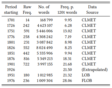
The grey line in Figure 8.1 shows Mair’s conservative estimate for the point at which the construction was firmly established as a way to express future tense.

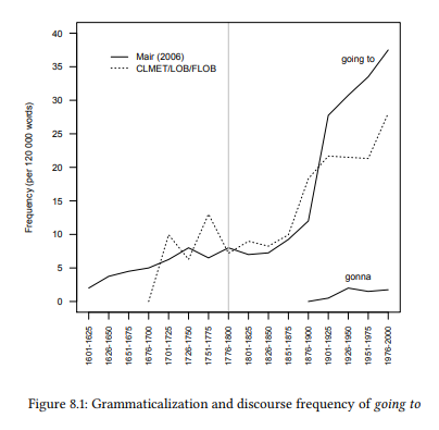
Figure 8.1: Grammaticalization and discourse frequency of going to

As the results from the OED citations and from the corpora show, there was only a small rise in frequency during the time that the construction became established, but a substantial jump in frequency afterwards. Interestingly, around the time of that jump, we also find the first documented instances of the contracted form gonna (from Mair’s data – the contracted form is not frequent enough in the corpora used here to be shown). These results suggest that semantic reanalysis is the first step in grammaticalization, followed by a rise in discourse frequency accompanied by phonological reduction.

This case study demonstrates that very large collections of citations can indeed be used as a corpus, as long as we are investigating phenomena that are likely to occur in citations collected to illustrate other phenomena; the results are very similar to those we get from well-constructed linguistic corpora. The case study also demonstrates the importance of corpora in diachronic research, a field of study which, as mentioned in Chapter 1 has always relied on citations drawn from authentic texts, but which can profit from querying large collections of such texts and quantifying the results.

8.2.6 Grammar and cultural analysis

Like words, grammatical structures usually represent themselves in corpus linguistic studies – they are either investigated as part of a description of the syntactic behavior of lexical items or they are investigated in their own right in order to learn something about their semantic, formal or functional restrictions. However, like words, they can also be used as representatives of some aspect of the speech community’s culture, specifically, a particular culturally defined scenario. To take a simple example: if we want to know what kinds of things are transferred between people in a given culture, we may look at the theme arguments of ditransitive constructions in a large corpus; we may look for collocates in the verb and theme positions of the ditransitive if we want to know how particular things are transferred (cf. Stefanowitsch & Gries 2009). In this way, grammatical structures can become diagnostics of culture. Again, care must be taken to ensure that the link between a grammatical structure and a putative scenario is plausible.

8.2.6.1 Case study: He said, she said

In a paper on the medial representation of men and women, Caldas-Coulthard (1993) finds that men are quoted vastly more frequently than women in the COBUILD corpus (cf. also Chapter 9). She also notes in passing that the verbs of communication used to introduce or attribute the quotes differ – both men’s and women’s speech is introduced using general verbs of communication, such as say or tell, but with respect to more descriptive verbs, there are differences: “Men shout and groan, while women (and children) scream and yell” (Caldas-Coulthard 1993: 204)

The construction [QUOTE + Subj + V] is a perfect example of a diagnostic for a cultural frame: it is routinely used (in written language) to describe a speech event. Crucially, the verb slot offers an opportunity to introduce additional information (such as the manner of speaking, as in the examples of manner verbs verbs just mentioned (that often contain evaluations), but also the type of speech act being performed (ask, order, etc.). It is also easy to find even in an untagged corpus, since it includes (by definition) a passage of direct speech surrounded by quotation marks, a subject that is, in an overwhelming number of cases, a pronoun, and a verb (or verb group) – typically in that order. In a written corpus, we can thus query the sequence〈[word="''"] [pos="pronoun"] [pos="verb"]〉 to find the majority of examples of the construction. In order to study differences in the representation of men and women, we can query the pronouns he and she separately to obtain representative samples of male and female speech act events without any annotation.

Table 8.27: Verbal collexemes of [QUOTE + Pron + V] (BNC)

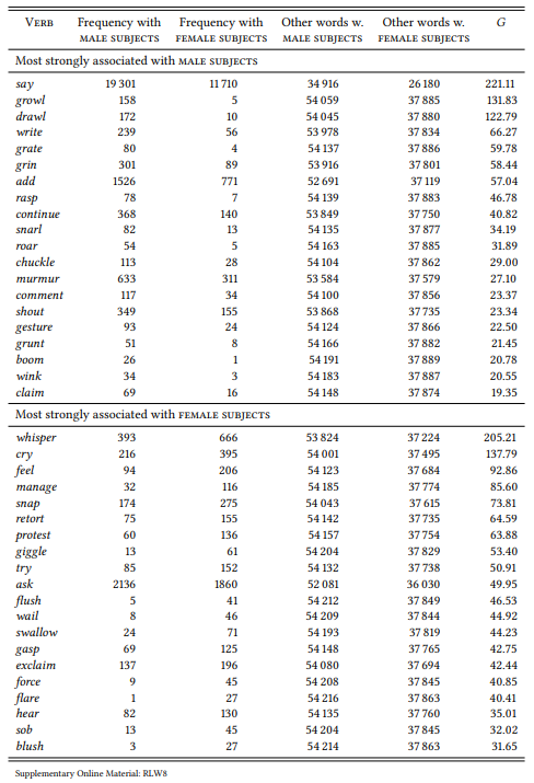
This design can be applied deductively, if we have hypotheses about the gender-specific usage of particular (sets of) verbs, or inductively, if we simply calculate the association strength of all verbs to one pronoun as compared to the other. In either case we have two nominal variables, SUBJECT OF QUOTED SPEECH, with the variables MALE (he) and FEMALE (she), and Speech Activity Verb with all occurring verbs as its values. Table 8.27 shows the results of an inductive application of the design to the BNC.

There is a clear difference that corroborates Caldas-Coulthard’s casual observation: the top ten verbs of communication associated with men contain five verbs conveying a rough, unpleasant and/or aggressive manner of speaking (growl, grate, rasp, snarl, roar), while those for women only include one (snap, related to irritability rather than outright aggression). Interestingly, two very general communication verbs, say and write, are also typical for men’s reported speech. Women’s speech is introduced by verbs conveying weakness or communicative subordination (whisper, cry, manage, protest, wail and deny).

8.2.7 Grammar and counterexamples

While this book focuses on quantitative designs, non-quantitative designs are possible within the general framework adopted. Chapter 3 included a discussion of counterexamples and their place in a scientific framework for corpus linguistics. Let us conclude this chapter with a case study making use of them.

8.2.7.1 Case study: To- vs. that-complements

A good case study for English that is based largely on counterexamples is Noël (2003), who looks at a number of claims made about the semantics of infinitival complements as compared to that-clauses. He takes claims made by other authors based on their intuition and treats them like Popperian hypotheses, searching the BNC for counterexamples. He mentions more or less informal impressions about frequencies, but only to clarify that the counterexamples are not just isolated occurrences that could be explained away.

For example, he takes the well-known claim that with verbs of knowing, infinitival complements present knowledge as subjective/personal, while that-clauses present knowledge as objective/impersonal/public. This is supposed to explain acceptability judgments like the following (Borkin 1973: 45–46, Wierzbicka 1988: 50, 136):

(15)     a. He found her to be intelligent.

   b. * I bet that if you look in the files, you’ll find her to be Mexican.

   c. I bet that if you look in the files, you’ll find that she is Mexican.

The crucial counterexample here would be one like (15b), with an infinitival complement that expresses knowledge that is “public” rather than “personal/ experiential”; also of interest would be examples with that-clauses that express personal/experiential knowledge. The corresponding queries are easy enough to define:

(16)     a. [word="(find|finds|finding|found)"%c] [word="(me|you|him| her|it|us|them)"%c] [word="to"%c] [word="be"%c]

   b. [word="(find|finds|finding|found)"%c] [word="that"%c] [word="(I|you|he|she|it|we|they)"%c] [word="(is|are|was| were)"%c]

This query follows the specific example in (15b) very narrowly – we could, of course, define a broader one that would capture, for example, proper names and noun phrases in addition to pronouns. But remember that we are looking for counterexamples, and if we can find these with a query following the structure of supposedly non-acceptable sentences very closely, they will be all the more convincing.

The BNC contains not just one, but many counterexamples. Here are some examples with that-complements expressing subjective, personal knowledge:

(17)     a. Erika was surprised to find that she was beginning to like Bach (BNC A7A)

   b. [A]che of loneliness apart, I found that I was stimulated by the challenge of finding my way about this great and beautiful city. (BNC AMC)

And here are some with to-complements expressing objective, impersonal knowledge:

(18)     a. Li and her coworkers have been able to locate these sequence variations ... in the three-dimensional structure of the toxin, and found them to be concentrated                in the β sheets of domain II. (BNC ALV)

   b. The visiting party, who were the first and last ever to get a good look at the crater of Perboewetan, found it to be about 1000 metres in diameter and about         fifty metres deep. (BNC ASR)

These counterexamples (and others not cited here) in fact give us a new hypothesis as to what the specific semantic contribution of the to-complement may be: if used to refer to objective knowledge, it overwhelmingly refers to situations where this objective knowledge was not previously known to the participants of the situation described. In fact, if we extend our search for counterexamples beyond the BNC to the world-wide web, we find examples that are even more parallel to (15b), such as (19), all produced by native speakers of English:

(19)     a. Afterwards found that French had stopped ship and found her to be German masquerading as Greek. (www.hmsneptune.com)

   b. I was able to trace back my Grandfathers name ... to Scotland and then into Sussex and Surrey, England. Very exciting! Reason being is because we were told         that the ancestors were Irish and we found them to be Scottish! (www.gettheeblowdryer.com)

   c. Eishaus – This place is an Erlangen institution, should you ever get to meet the owner you’ll find him to be American, he runs this wonderful ice cream shop as        his summer job away from his ‘proper’ job in the states. (theerlangenexpat.wordpress.com)

Again, what is different in these examples from the (supposedly unacceptable) example (15b) is that the knowledge in question is new (and surprising) to the participants of the situation – a seemingly Greek ship turning out to be German, a supposedly Irish ancestor turning out to be Scottish, and the proprietor of an ice-cream shop in the small Bavarian town of Erlangen turning out to be America.

This observation could now be used as the basis for a new hypothesis concerning the difference between the two constructions, but even if it is not or if this hypothesis turned out to be false, the counterexamples clearly disprove the claim by Wierzbicka and others concerning the subjective/objective distinction (Noël 2003 actually goes on to propose an information-structural account of the difference between the to- and the that-complement).

This case study was intended to show how counterexamples may play a role in disproving hypotheses based on introspection and constructed examples (see Meurers 2005 and Meurers & Müller 2009 as good examples for the theoretically informed search for counterexamples).

 

¹ Unlike in the rest of the book, I have to use data from a corpus that is not generally accessible – the British Component of the International Corpus of English. The reason is that analysis like the ones presented here require a treebank (see Section 2.1.4 in Chapter 4), and there is no sufficiently large and generally accessible treebank.